A preconditioned method for saddle point problems(Mathematical Sciences for Large Scale Numerical Simulations)

A preconditioned method for saddle

point

problems

Kouji Hashimoto

Graduate SchoolofInformatics, Kyoto University, Kyoto 606-8317, Japan.

hashimot@amp.i.kyoto-u.ac.jp

Abstract

Apreconditionedmethod for saddlepoint problems is presented andanalyzed. We showa

double preconditioned method forspecialsaddlepoint problems, andapplythe newmethod

tosome standarditerativesolution methods. The method isillustratedby several examples

derived $hom$ the surface fittingproblems. Preliminary numerical results indicate that the

method is efficient.

AMSSubject

_{Classifications:}

$65F10$

,

65N25

Keyword: Saddle Point Problem, Double Preconditioned Method, Surface Fitting Problem

1

Introduction

In this paper,

we

consider the followingsaddle point problems.

$(\begin{array}{ll}\mathcal{A} B^{T}B 0_{m}\end{array})(\begin{array}{l}xy\end{array})=(\begin{array}{l}fg\end{array})$ (1.1)

where $\mathcal{A}$ is

an

$nxn$ symmetric and positive semi-definite matrix, $B$ is

an

$mxn$ matrix and

$f\in R^{n},$ $g\in R^{m}$

are

given vectors. It is assumed that $n\geq m$

.

The problem (1.1) $arise8$ in the partial differential equations and optimization problems

([12][14]) and usually becomes large systems. The matrix in (1.1) is known

as

a

saddle point

matrix which is

an

indefinite matrix. In general,

a

numericalsolution method for the indefinite

problem is theoretically difficult comparedwith positive definite problems, andthe

convergence

rate becomes slow. Recently, preconditioned

Uzawa

algorithms

are

studied ([3][5][6][8]) and

are

shown

as

an

effective

iterative solution method

for

the saddle point problem. Under

some

assumptions, these algorithms will be devised by using theouter iteration. Then

we can

refor-mulate the coefficient matrix (1.1) as a symmetric and positive definite problem.

1.1

The unique solvability

Let $U$ be

an

$mxm$ symmetric and positive

definite

matrix. We know that if $(A, B^{T})$ has

full-row rank, that is, $r\bm{t}k(\mathcal{A}, B^{T})=n$ then $\mathcal{A}_{U}\equiv \mathcal{A}+B^{T}UB$ is positive definite. Hence

we

now

consider the followingsaddle point problems.

$(\begin{array}{ll}A_{U} B^{T}B 0_{m}\end{array})(\begin{array}{l}xy\end{array})=(\begin{array}{l}f_{U}g\end{array})$ (1.2)

Since (1.1) is equivalent to (1.2),

we

generally know that if $\mathcal{A}_{U}$ and $S_{U}\equiv B\mathcal{A}_{U}^{-1}B^{T}$

are

positive definite then (1.1) has

a

unique solution. Then

an

exact solution $(x^{*}, y^{*})$ of (1.1) is

written by

$y^{*}$ $=$ $S_{U}^{-1}(B\mathcal{A}_{U}^{-1}f_{U}-g)$,

(1.3)

$x^{*}$ _$=$ $\mathcal{A}_{U}^{-1}(f_{U}-B^{T}y^{*})$

.

Notice that for the formula (1.3),

we

can easily solve the second equation since$n\geq m$

.

In this

paper,

we

consider the preconditioned method for the first equation (linear system $S_{U}$).

1.2 Motivation and

Purpose

During the years, much raeearch has been devoted to inner

iterative

solution methods for

sym-metric and positive definite problems $([1][11])$, then $the8e$ preconditioned methods

are

fast.

Moreover, thepreconditioned methodfor thesaddlepoint problemis

also

$pr\infty ented([2][3][4][9])$

.

For almost mathematical modek of physical and natural phenomena, using the finite

ele-$ment/difference$ method with amaeh size $h>0$

,

we

generally know that the cost (time) for

numerical computations is increasing when $h$ is decreasing. For example, if

we use

aprecondi-tioner for discretizationsby the incomplete Cholesky decompositionwith afixed tolerance then

the iteration number is also increasing. It

meao

that atotal computing cost depends

on

the

dimensionand iterationnumbers. Note that the condition number influences theiteration

num-ber. Thus, if

we

assume

that the condition number is

a

$con8tant$ independent ofthe mesh size

$h$ then

we

can

easily $\infty timate$ the total cost of numerIcal computations for large systems. Note

that the saddle point problem is reduced to the linear system $S_{U}hom(1.3)$

.

Of

course, if

we

take thepreconditioner

as

the inverse matrix then the condition number is always

one.

However,

we

expect that it isdifficult for the linearsystem $S_{U}$ togenerate agood preconditioner, because

$S_{U}$ is not give and is generally dense. Hence

we

consider adouble preconditioned method to

give agood condition number independent ofthe dimeoionwithout using $\mathcal{A}_{U}^{-1}$

.

Here

we

only show the preconditioned CGmethod ofthe Uzawa-type below.

Algorithm 1 (Q-Preconditioned $CG$ Method

of

the Uzawa-type)

For

an

initialguess $y_{0}$,

Solve $x_{0}=\mathcal{A}_{U}^{-1}(f_{U}-B^{T}y_{0})$;

Compute $r_{0}=Bx_{0}-g$; $p_{0}=Q^{-1}r_{0}$;

For $k=0$ to

convergence

Solve

$[Sp]_{k}=BA_{U}^{-1}B^{T}p_{k}$;

Compute $y_{k+1}=y_{k}+\alpha_{k}p_{k}$; where $\alpha_{k}=(r_{k},p_{k})/(p_{k}, [Sp]_{k})$;

Compute $r_{k+1}=r_{k}-\alpha_{k}[Sp]_{k}$;

Solve

$u=Q^{-1}r_{k+1}$;

Compute $p_{k+1}=u-\beta_{k}p_{k}$; where $\beta_{k}=(u, [Sp]_{k})/(p_{k}, [Sp]_{k})$;

End

Solve $x_{k+1}=\mathcal{A}_{U}^{-1}(f_{U}-B^{T}y_{k+1})$;

Since many saddle point problems of mathematical models satisfy that there exists

a constant

$M>0$ independent ofthe dimension$n$ such that $||A||_{2}\leq M$

,

if

we

take preconditioners $U$ and

$Q$ satisfying $cond_{2}(Q^{-}1rS_{U}Q^{-1}2)<1+\epsilon\Vert A\Vert_{2}$

,

where $1\gg\epsilon>0$ (independent ofn) then it

becomes

a

fast solution method forlarge saddle point systems.

Therefore,

our

purpose

of this paper is to take good preconditioners $U$ and $Q$

,

and apply

We denote the largest and smallest eigenvalues of

a

matrix by $\lambda_{\max}(\cdot)$

and

$\lambda_{lni\mathfrak{n}}(\cdot)$

,

respec-tively. Moreover, $\rho(\cdot)$ and $cond_{2}(\cdot)$ denote

a

spectral radius and condition number with respect

to 2-norm, respectively. Also $I_{k}$ denotes the k-th identity matrix and $0_{k}\equiv 0\cdot I_{k}$

.

For the

discussion,

we assume

that $B$ has full-row rank, that is, rank$(B)=m$

.

2

The preconditioned

method

In this section,

we

discuss

a

preconditioned method for the saddle point problems (1.1), and

we

aesume

that $A_{U}\equiv A+B^{T}UB$ _{is positive definite and} $B$ has full-row rank, it implies that

the matrix $S_{U}\equiv BA_{U}^{-1}B^{T}$ is also positive definite. For

our

problems, it is important for the

convergence

ofiterative solution methods to analyze the property of$S_{U}$

.

Usually,

we

want to

take the preconditioner

as

approximations of$S_{U}^{-1}$

,

however, $S_{U}$ is not

a

given matrix. Hence

we

introduce

an

effective preconditioned

method

without using $\mathcal{A}_{U}^{-1}$

.

Here

we

show

a

standard preconditionedmethod for the problem (1.2). Let $Q$ be

an

$mxm$

symmetricandpositivedefinite matrix. Then (1.2) isequivalent

to

thefollowingpreconditioned

problems.

$(\begin{array}{ll}I_{n} 00 Q^{-\}\end{array})(\begin{array}{ll}\mathcal{A}_{U} B^{T}B 0_{m}\end{array})(\begin{array}{ll}I_{n} 00 Q^{-l}2\end{array})(\begin{array}{ll}x Q\} y\end{array})=(\begin{array}{l}f_{U}Q^{-A}2g\end{array})$

.

(2.1)

Let $V$ and $W$ be _$mxm$symmetric and positive definite matrices. If_$A+B^{T}VB$ is _positive

definite and $B$ has full-row rank then

we

have the following equality which

was

presented by

Golubet al. in [9].

$(B(\grave{A}+B^{T}VB)^{-1}B^{T})^{-1}=(B(\mathcal{A}+B^{T}(V+W)B)^{-1}B^{T})^{-1}-W$

.

_(2.2)

First

we

briefly discuss

a

single preconditioned method for (1.2). From (2.2),

we

have

$cond_{2}(WS_{(V+W)}W^{A}2=\frac{\lambda_{\min}(WS_{V}W)+1}{\lambda_{\max}(WaS_{V}WAi)+1}cond_{2}(WS_{V}W)$

,

(2.3)

where $S_{V}\cong BA_{V}^{-1}B^{T}$

.

Thus if

we

take $V=\kappa_{1}I_{m}$ and $W=\kappa_{2}I_{m}$ then it implies that

$cond_{2}(S_{(\kappa_{1}I_{m}+\kappa_{2}I_{m})})=\frac{\lambda_{\min}(S_{(\kappa_{1}I_{m})})+\kappa_{2}^{-1}}{\lambda_{mu}(S_{(\kappa_{1}I_{m})})+\kappa_{2}^{-1}}cond_{2}(S_{(n_{1}I_{n})})$

,

where$\kappa_{1}$ and $\kappa_{2}$

are

positive constants. Henoe if

we

take$\kappa_{2}$ satisfying $\kappa_{2}\cdot\lambda_{\min}(S_{(\kappa_{1}I_{m})})\cdot\gg 1$ for

a

fixed $\kappa_{1}$ then $U=(\kappa_{1}+\kappa_{2})I_{m}$ becomes

a

good preconditioner for (1.2).

Next

we

consider

a

double preconditioned method. Notice that matrices $U$ and $Q$ in (2.1)

become

the first and second preconditioners, respectiveiy.

As

a

similar argument, if

we

take $V$

and $W$satisfying $\lambda_{\min}(W\# s_{V}W^{\frac{1}{l}})\gg 1$ then _$V$and _$W$ become good preconditioners. Here

we

show thefollowing result which

was

presented by Chen and the author in [7].

Lemma 2 Let $S\equiv BA^{-1}B^{T}+C$, where $A$ is an$nxn$ symmetric and positive

definite

matrix,

$C$ is

an

_$mxm$ symmetric andpositive

semi-definite

matrix.

If

$B$ has

full-row

rankthen

we

have

$\Vert L^{T}S^{-1}L\Vert_{2}\leq\frac{||A||_{2}}{1+\lambda_{\min}(L^{-1}CL^{-T})||A\Vert_{2}}$

,

Using above lemma,

we

show the following main results of this paper.

Theorem 3 (Double: $U=\kappa Q^{-1},$ $Q=BB^{T}$_{) Assume that} $(A, B^{T})$ and $B$ have

full-row

rank.

Then we have

$cond_{2}((BB^{T^{1}T^{1}})^{-f}S_{(\kappa(BB^{T})^{-1})}(BB)^{-f})<1+\kappa^{-1}\Vert A||_{2}$

,

where $\kappa$ is

a

positive constant.

Proof: For (2.3), if

we

take $W=\kappa_{2}(BB^{T})^{-1}$ then it implies that

$cond_{2}(W^{1}zS_{(V+W) ,\}}W^{1}z)cond_{2}(2$ $=$ $\frac{cond_{2}((BB^{T})^{-}z1S_{(V+\kappa_{2}(BB^{T})^{-1})}(BB^{T})^{-\frac{1}{2}})}{Cond_{2}(2}$

$=$ $\frac{\lambda_{\min}((BB^{T})^{-p}1S_{V}(BB^{T})^{-:})+\kappa_{2}^{-1}}{\lambda_{\max}((BB^{T})^{-\}}S_{V}(BB^{T})^{-:})+\kappa_{2}^{-1}}$

Then usingLemma 2,

we can

obtain the following estimation.

$\lambda_{\min}((BB^{\tau^{\iota\iota}})^{-\pi}S_{V}(BB^{T})^{-f})\geq\frac{1}{\Vert \mathcal{A}_{V}\Vert_{2}}$

.

Hence it implies that

$\lambda_{\min}((BB^{T^{1}})^{-f}S_{V}(BB^{T})^{-\#})+\kappa_{2}^{-1}\leq\lambda_{\min}(2(1+\kappa_{2}^{-1}||A_{V}\Vert_{2})$

.

Since $\kappa_{2}$ is positive, if

we

take$V=\kappa_{1}(BB^{T})^{-1}$ then it impiesthat

$cond_{2}((BB^{T})^{-\Delta}2S_{((\kappa_{1}+\kappa_{2})(BB^{T})^{-1})}(BB^{T})^{-:})<1+\kappa_{2}^{-1}\Vert A_{(\kappa_{1}(BB^{T})^{-1})}\Vert_{2}$

.

Moreover,

we can

obtain

$\Vert A\tau-1$ $=$ $\Vert \mathcal{A}+\kappa_{1}B^{T}(BB^{T})^{-1}B\Vert_{2}$

$\leq$ $\Vert \mathcal{A}\Vert_{2}+\kappa_{1}$,

which

follows

that the largest eigenvalue of $B^{T}(BB^{T})^{-1}B$ is equal to

1.

Therefore, taking

$\kappa\equiv\kappa_{1}+\kappa_{2}$ and $\kappa_{1}arrow 0$, this proofis completed. $\blacksquare$

Corollary 4 (Single; $U=\kappa Q^{-1},$ _{$Q=I_{m}$})[$9J$ Assume that $(A, B^{T})$ and $B$ have

full-row

rank.

Then$cond_{2}(S_{(\kappa I_{m})})$ is strictly decreasing, that is, $cond_{2}(S_{(\kappa I_{m})})arrow 1$

as

$\kappaarrow\infty$

.

Here

we

can

write matrices $\mathcal{A}$and $B$ by

$\mathcal{A}=(\begin{array}{ll}A_{*} \mathcal{A}_{\perp}^{T}A_{\perp} \mathcal{A}_{o}\end{array})$ $B=(B_{o},B_{n})$

,

respectively. It is assumed that $A_{*},$ $A_{o}$ and $B_{n}$

are

square,

and $\dim(A_{o})=\dim(B_{*})=m$

.

If

$\mathcal{A}_{1}\neq 0$ then the computing

cost

of$cond_{2}(A)$ and $cond_{2}(\mathcal{A}_{U})$ in Theorem ?? is almost

same.

Thus

as

a

special case,

we

show the following estimate.

Corollary 5 Assume that$\mathcal{A}\perp=0$

,

that is, $\mathcal{A}=diag(A_{*},\mathcal{A}_{o})$

. If

$A_{*}$ is positive

definite

and$B_{*}$

is nonsingularthen we have

Proof: Since $\Vert A_{U}^{-1}\Vert_{2}=\lambda_{\min}(\mathcal{A}_{U})^{-1}$ and (diag$(A_{*},$ $0_{m}),$$B^{T}$) has full-row rank,

we

have

$\lambda_{\min}(\mathcal{A}_{U})$ $=$ $\lambda_{\min}((\begin{array}{ll}\mathcal{A}_{*} 00 \mathcal{A}_{o}\end{array})+($ $B_{o}^{T}UB_{o}B_{*}^{T}UB_{o}$ $B_{o}^{T}UB_{*}B_{*}^{T}UB_{*}$

)

_$)$ $\geq$ $\lambda_{m\ln}((\begin{array}{ll}\mathcal{A}_{*} 00 0_{m}\end{array})+(B_{o}^{T}UB_{o}B_{*}^{T}UB_{o}$ $B_{*}^{T}UB_{*}B_{o}^{T}UB_{*}))$

$=$ $\lambda_{\min}$

((

$I_{(n-m)}$

$B_{o}^{T}B_{*}^{T}$

)

$(\begin{array}{ll}\mathcal{A}_{*} 00 U\end{array})(\begin{array}{ll}I_{(n-m)} 0B_{o} B_{*}\end{array})$

).

Therefore, this proof is completed. $\blacksquare$

Corollary 6

_If

$U=\kappa(BB^{T})^{-1}$ then

we

have $||\mathcal{A}_{(\kappa(BB^{T})^{-1})}\Vert_{2}\leq\Vert A\Vert_{2}+\kappa$

.

Proof: Since the largest eigenvalueof$B^{T}(BB^{T})^{-1}B$ is equal to 1, this proofiscompleted. $\blacksquare$

3

Numerical

examples

In this section,

we

report Iome numerical results for the preconditioned method to solve the

saddle point problems. Let $\Omega\subset R^{2}$ be

a

bounded and open domain. We denote the usualk-th

order $L^{2}$ Sobolev space

on

$\Omega$ (notethat $(x,y)\in R^{2}$)by $H^{k}(\Omega)$ anddefine $(\cdot, \cdot)_{L^{2}}$

as

the $L^{2}$ inner

product. We also consider the following

some

Sobolev spaces.

$H_{0}^{1}(\Omega)$ $\equiv$

{

$v\in H^{1}(\Omega)$ ; $v=0$

on

$\partial\Omega$

},

$H_{0}^{2}(\Omega)$ $\equiv$

{

$v\in H^{2}(\Omega)$ ; $v=\nabla_{x}v=\nabla_{y}v=0$

on

$\partial\Omega$

}.

Let $X_{h}\subset H_{0}^{1}(\Omega)$ be

a

finite element subspacewhichdepends

on

a

parameter $h$

,

and let $\{\varphi_{1}\}_{i=1}^{m}$

be thebasis of$X_{h}$

.

3.1

The

surface

fitting

problems

Consider the following surface fittingproblems.

min $\nu||\Delta u\Vert_{L^{2}}^{2}+\Vert u(z)-f\Vert_{2}^{2}$

,

(3.1)

$u\in H_{0}^{2}(\Omega)$

where$z=(z_{1}^{(1)}, z_{i}^{(2)})\in R^{ex2},$ _{$f=(f_{i})\in R^{c}$}

are

given vectors and_$\nu>0$isa_{relaxationparameter.}

Since $u\in H_{0}^{2}(\Omega),$ $\nabla_{x}u,$ $\nabla_{y}u$ and $u$ belong to $H_{0}^{1}(\Omega)$

.

Thus using the $H^{1}$-method ([12]),

an

approximate problem of (3.1) isgiven by

$\min$ $\nu\Vert\nabla u_{h}^{(1)}\Vert_{L^{2}}^{2}+\nu\Vert\nabla u_{h}^{(2)}\Vert_{L^{2}}^{2}+\Vert u_{h}^{(3)}(z)-f\Vert_{2}^{2}$

,

$u_{h}^{(1)},u_{h}^{(2)},u_{h}^{(S)}\in x_{h}$ (3.2)

subject to $(\nabla u_{h}^{(3)}, \nabla v_{h})_{L^{2}}=(-div(u_{h}^{(1)},u_{h}^{(2)}),v_{h})_{L^{2}}$ _{$\forall v_{h}\in X_{h}$}

.

Then using thesolutions$u_{h}^{(1)},$ $u_{h}^{(2)},$$u_{h}^{(3)}\in X_{h}$ and$u_{h}^{(4)}\in X_{h}$,

we

can

take

an

approximate solution

$u_{h}\in H_{0}^{2}(\Omega)$ of (3.1) by the Hermite spline functions ([13]), where$u_{h}^{(4)}\in X_{h}$ satisfies $(u_{h}^{(4)},v_{h})_{L^{2}}= \frac{1}{2}(div(u_{h}^{(2)},u_{h}^{(1)}),v_{h})_{L^{2}}$ $\forall v_{h}\in X_{h}$

.

Let matrices $A_{1}=(a_{ij}^{(1)})\in R^{mxm},$ $A_{3}=(a_{ij}^{(3)})\in R^{cxm}$ and $B_{1}=(b_{ij}^{(1)}),$ $B_{2}=(b_{ij}^{(2)})\in R^{mxm}$

have the entries

$a_{ij}=\varphi_{j}(z_{i}^{(1)}, z_{i}^{(2)})a_{i}^{(1)}j_{3)}=(\nabla\varphi_{j},\nabla\varphi_{i})_{L^{2}}$

,

$b_{ij}i_{2)}=(\nabla_{y}\varphi j\varphi_{i})_{L^{2}}b_{9}^{(1)}=(\nabla_{x}\varphi_{j}, \varphi_{i})_{L^{2}}$

,

respectively. $(n=3m)$ In this example,

we

choose the basis for the finite element subspace $X_{h}$

as

piecewise bi-linear functions for the uniform and squaremesh. Then letting $A_{2}=B_{3}=A_{1}$,

the problem (3.2) has the following saddle point form.

(3.3)

Notice that if $c<m$ then $A_{3}^{T}A_{3}$ is always positive 8emi-definite. Thus

we

cannot

assume

that

$A_{3}^{T}A_{3}$ is positive

definite.

However, this example

satiIfies that

_{$(A, B^{T})$}

and

$B$

have

$fullarrow row$

rank since $B_{3}=A_{1}$

,

where $A:=diag(\nu A_{1}, \nu A_{2}, A_{3}^{T}A_{3})$ and $B:=(B_{1}, B_{2}, B_{3})$

.

Henoe using

techniquesofSection 1.1,

we reformulate

(3.3)

as

$(\begin{array}{ll}A+B^{T}UB B^{T}B 0_{m}\end{array})(\begin{array}{l}x_{l}x_{2}\frac{x_{3}}{y}\end{array})=(\begin{array}{l}00\frac{A_{3}^{T}f}{0}\end{array})$

.

Here we briefly consider a linear system $\mathcal{A}_{U}\equiv \mathcal{A}+B^{T}UB$ for this example. For the surface

fitting problems,

we

expect that if $harrow 0$ then $A_{3}^{T}A_{3}$ becomes sparse, it implies that $A_{U}\approx$

diag$(A_{*}, 0_{m})+B^{T}UB$

,

where$A_{*}:=diag(\nu A_{1}, \nu A_{2})$

.

Thussetting$B_{o}$ $:=(B_{1}, B_{2})$

,

the following

matrix will become

a

good preconditioner for the linear system $A_{U}$ since the matrices satisfy

the assumption in Corollary

5.

$(\begin{array}{ll}\mathcal{A}_{*} 00 0_{m}\end{array})+B^{T}UB=($ $I_{(n-m)}$ $B_{3}^{T}B_{o}^{T}$

)

$(\begin{array}{ll}A_{*} 00 U\end{array})(I_{(n-m)}$ $B_{3}0)$

.

3.2

Numerical

results

In this section,

we

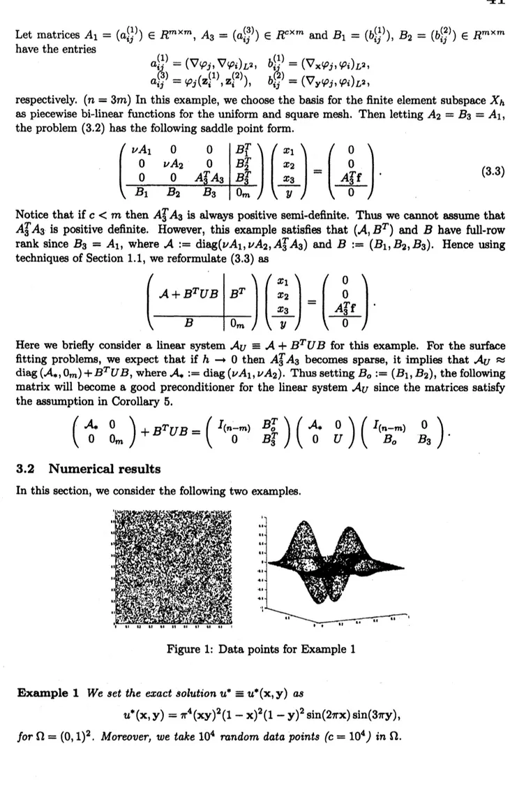
consider the following two examples.

Figure

1:

Data points for Example

1

Example 1 We set the exact solution $u^{*}\equiv u^{*}(x,y)$

as

$u^{*}(x,y)=\pi^{4}(xy)^{2}(1-x)^{2}(1-y)^{2}\sin(2\pi x)\sin(3\pi y)$

,

Example 2 We use real data $(c=327)$

_of

Niigata

_Prefecture

Chuetsu Earthquake which

was

happened at

17:56

in October 23,

₂₀₀₄

($S7.291N,$ $lS8.867E$, lSKm, M6.8), and take $\Omega=$

$(135,34)x(142,41)$

.

Note that

we

take data $z=(z_{i}^{(1)},z_{i}^{(2)})$ and _{$f=(f_{i})$}

as

(East longitude,

North latitude) and the maximum acceleration $(gal)$ at the station point, respectively. Moreover,

the maximum value

_of

data $f$ is

1307.911.

This data is supported byK-Net in National Research

Institute

_for

Earth Science and DisasterPrevention.

First

we

show

some

norms

for Examples 1 and 2 in Tables 1 and 2, respectively. Note that

computed minimum eigenvalues of $A_{3}^{T}A_{3}$ for $h^{-1}=80$

, 100

inTable 1

are

less than $2^{-52}$

.

From abovetables,

we can

assume

that $\Vert \mathcal{A}\Vert_{2}=\max\{\nu\cdot\lambda_{\max}(A_{1}), \lambda_{\max}(A_{3}^{T}A_{3})\}$ isthe constant

independent of the dimension. Hence

we

expect that

our

preconditioned methods lead good

(effective) condition numbers for bothexamples.

Therefore,

we

next show

the

condition number

$Cond_{2}(Q^{-i_{S_{U}Q^{-}7)}^{1}}$

for

Example

1

in Figure

2.

For $\nu=10^{-2}$

,

the left-hand side and right-hand

side

_{in Figure}

2

_{show several results for}

$U=\kappa Q^{-1}$ and $U\neq\kappa Q^{-1}$, respectively.

Note

that $U\neq\kappa Q^{-1}$

means

if $Q=BB^{T}$ and _{$Q=I_{m}$}

then $U=\kappa I_{m}$ and $U=\kappa(BB^{T})^{-1}$, respectively.

Figure 2; $cond_{2}(Q-1lS_{U}Q^{-\int})$ for _Example 1 for $\kappa=10$

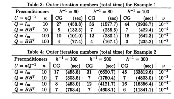
Finally

we

show numerical results for Examples 1 and 2 by the preconditioned

CG

method

(CG: Algorithm 1) in Tables 3 and 4, respectively. We apply the single and double

precon-ditioned methods to the $case8h^{-1}=60,80$,

100

for Example 1 and $h^{-1}=100,200$_,

₃₀₀

_for

Notethat

we

use

the direct method (Complete Cholesky Decomposition and

Gaussian

Elimina-tion) for linear systems $A_{1}(A_{3}^{T}A_{3})$ and $BB^{T}$

.

Moreover, for the linear system $\mathcal{A}+B^{T}UB$

,

we

use

thepreconditioned

CG

method with respect to thecriterion $\delta$ of the relativeresidual error,

that is, $\delta<10^{-12}$

.

We

only show

an

approximation of Example

2

for _$h^{-1}=300$

in

Figure

3.

Figure

3:

An

approximationfor Example

2

for $\nu=10^{-4}$

All computations intables and figures

are

carriedout

on

theDellPrecision 650 Workstation

Intel XeonCPU

3.

$20GHz$ _by

MATLAB.

Conclusion

We have proposed

a

good preconditioner and double preconditioned method for saddle point

problems,andshown the actual effectiveness to numerical computations. Comparingother case,

our

methods lead

a

few iteration numbers independent of the dimension by

numerical

results.

Of course, when

we

take $U=\kappa BB$ then

a

cost for

one

time iteration is

more

expensive than

the

case

$U=\kappa I_{m}$

.

However, total computing cost for the former is much less than the latter,

Acknowledgement

The author is grateful to Professor Xiaojun Chen for herveryhelpfulcomments and suggestion.

This work is supported by The Japan Society for Promotion ofScience (JSPS) and National

Research Institute forEarth Science andDisasterPrevention (NIED).

References

[1] O. Axelsson; Iterative Solution Methods, CambridgeUniversity Press, London,

1996.

[2] $0$

.

Axelsson and M. Neytcheva; Eigenvalue estimates for preconditioned saddle point

ma-trices,

Numer.

Linear Algebra Appl.

13

(2005),

pp.

339-360.

[3] M. Benzi, G. H. Golub, and J. Liesen; Numerical

Solution

ofSaddle Point Problems,

Acta

Numerica, 14 (2005), pp.

1-137

[4] M.A. Botchev and G.H. Golub; A class of nonsymmetric preconditioners for saddle point

problems, $S\mathcal{U}M$J. Matrix Anal.

27

(2006), pp.

1125-1149.

[5] J. Bramble, J. Pasciak and A. Vassilev; Analysis of theinexact Uzawaalgorithm for saddle

point problems, SIAM$J$

.

Numer. Anal. 34 (1997), pp. 1072-1092.

[6] X. Chen; Onpreconditioned Uzawa methods and

SOR

methods for saddle point problems,

J. Comp. Appl. Math.

100

(1998), pp.

207-224.

[7]

X.

Chen and K.

Hashimoto; Numerical

_{validation of solutions of saddle}

point

matrix

equa-tions, Numer. Linear Algebra Appl.

10

(2003), pp. $661arrow 672$

.

[8] H.C. Elman and

G.H.

Golub;

Inexact

andpreconditioned

Uzawa

algorithm for saddlepoint

problems, SLAM J. Numer. Anal. 31 (1994), pp.

1645-1661.

[9] G.H. Golub, C. Greifand J.M. Varah; An algebraic analysis of

a

block diagonal

precondi-tioner for saddle point systems, SIAMJ. MatrixAnal.

27

(2006), pp.

779-792.

[10] G.H. Golub and C.F. Van Loan; Matrix Computations, Johns Hopkins University Press,

Baltimore, second edition,

1989.

[11] A. Greenbaum, Iterative Methods

for

Solving

Linear

Systems (Frontiersin Applied

Math-ematics

Vol.17), SIAM, Philadelphia, PA.,

1997.

[12]

M.

Hegland,

S. Roberts and I.

Altas; Finite

element

thin plate splines

for

surface fitting,

Computational Tbchniques

an

$d$Applications

CTAC97

WorldScientific (1997),pp.

289-296.

[13] M.H. Schultz; Spline Analysis, Prentice-Hall, London,

1973.

[14] M. Tabata andD. Tagami; A finite element analysis of

a

linearized problem of the