On the use of the QMR_SYM method for solving complex symmetric shifted linear systems (High Performance Algorithms for Computational Science and Their Applications)

On

the

use

of the

QMR-SYM method for solving

complex

symmetric

shifted linear systems

名古屋大学大学院工学研究科 曽我部知広 (Tomohiro Sogabe)

Graduate school ofengineering, Nagoya University

名古屋大学大学院工学研究科 張紹良 (Shao-Liang Zhang)

Graduate school ofengineering, Nagoya University

Abstract

We consider the solution of complex symmetric shifted linear systems. Such

systems arise in large scale electronic structure theory and there is a strong need

for the fast solution of the systems. Since the QMR-SYM method is known as

a powerful solver for complex symmetric linear systems, we use the idea of the

QMR-SYM method together with shift-invariant property of the Krylov subspace for solving complex symmetric shifted linear systems.

1

Introduction

In this paper

we

consider the solution of complexsymmetric shifted linear systems of the form

$(A+\sigma_{l}I)x^{(l)}=b$, $\ell=1,2,$ _$\ldots,$$m$, (1)

where $A$(ae) $:=A+\sigma_{\ell}I$

are

nonsingular N-by-N complex symmetric sparse matrices, i.e.,

$A(\sigma_{\ell})=\mathcal{A}(\sigma_{\ell})^{T}\neq\overline{A}(\sigma_{\ell})^{T}$, withscalar shifts $\sigma_{\ell}\in C,$ $I$ is the N-by-N identity matrix, and

$x^{(\ell)},$$b$

are

complex vectors oflength $N$. The above systems arise in large-scale electronic

structure theory [14] and there is

a

strong need for the fast solution of the systems.

Since the given shifted linear systems (1) are a set of sparse linear systems, it is

natural to

use

Krylov subspace methods, and

moreover

since the coefficient matrices

are

complex symmetric,

one

ofthesimplest ways to solve the shifted linearsystems is applying

(preconditioned) Krylov subspace methods for solving complex symmetric linear systems

such as the COCG method [15], the COCR method [12], and the QMR-SYM method [2] to all of the shifted linear systems (1). On the otherhand, denoting n-dimensional Krylov

subspace with respect to $A$ and $b$ as _{$K_{n}(A, b)$ $:=$} span_{$\{b, Ab, . . . , A^{n-1}b\}$},

we

observe that

$K_{n}(A, b)=K_{n}(A(\sigma_{\ell}), b)$

.

(2)

This implies that

once

Krylov basis vectors

are

generated from

one

of Krylov subspaces

$K_{n}(A(\sigma_{\ell}), b)$, these basis vectors

can

be used to solve all the shifted linear systems. In

other words, there is

no

need to generate all Krylov subspaces $K_{n}(A(\sigma_{\ell}), b)$, and thus

computational costs involving the basis generation, e.g., matrix-vector multiplications,

are

saved. Here we give a concrete example: if

we

apply the COCG method to all of

the linear systems (1), then $K_{n}(A(\sigma_{\ell}), b)$ for $\ell=1,2,$

$\ldots,$$m$

are

generated. On the other

as the “seed system”), then the Krylov basis vectors are generated from the seed system

and these vectors are used to solve the rest of the shifted linear systems.

Based

on

the observation (2), the shifted conjugate orthogonal conjugate gradient

(shifted COCG) method has been recently proposed [14]. The shifted COCG method

works well for the problems from _{electronic structure} theory. However, theshifted COCG

method requires the choice of

a

seed system, the term $\zeta seed$ system”

was

mentioned

in the previous _{paragraph, and unsuitable choice may lead to the drawback that many}

shifted linear systems _{remain unsolved. To avoid the drawback,}

_more

_{recently, the seed}

switching technique has been proposed [13]. For

some

problems _{from electronic structure}

theory, it has been shown that the shifted COCG method together withthe seed switching

technique is practical.

There is another approach to solving the shifted linear systems (1). That is the

use

of Krylov subspace methods for non-Hermitian shifted linear systems such as the shifted

BiCGStab$(\ell)$ method [5], the shifted (TF)QMR method [3], the

restarted shifted FOM

method [9], and the restarted shifted

GMRES

method [6],

see

also, e.g., [10]. We readily

see that the relation (2) holds not only for complex symmetric _{matrices but also for}

non-Hermitian matrices, and these methods

are

based on the

use

of this shift-invariant

relation. Therefore, this

can

be

a

good approach. However, since these methods do not

exploit the property of complex symmetric matrices, these computational costs

can

be

more

expensive than that ofthe shifted

COCG

method.

The shifted COCG method is obtained from the COCG method and the COCG

method is closely related to the QMR-SYM method, see [2, Prop. 3.3]. Hence, it is

nat-ural _{to consider algorithms using the QMR-SYM method for solving complex symmetric}

shifted linear systems. The main purpose of the present paper is to develop variants of

the QMR$arrow SYM$ method by considering the minimization ofweighted_{quasi-residual}

norms

for solving complex symmetric shifted linear systems. Of many possible choices ofweight

matrices for the norms,

we

will show that there exists

a

practical weight when the number

$m$ of shifted linear systems

are

large enough.

The present paper is organized as follows: in the next section, an algorithm (referred

to

as

shifted QMR-SYM) for solving the systems (1) will be derived from two important

results given by Freund [2, 3], and some properties of the shifted QMR-SYM method

are given for the problem from large-scale electronic structure theory. In section 3, some

results of

a

numerical example from electronic structure theory

are

shown to

see

the

performance of the shifted QMR-SYM approach. Finally,

some

concluding remarks are

made in section 4.

Throughout this paper, unless otherwise stated, all vectors and matrices

are

assumed

to be complex. $\overline{M},$ $M^{T},$ $M^{H}=\overline{M}^{T}$ denote the complex conjugate, transpose, and

Hermitian matrix of the matrix M. $\Vert v\Vert_{W}$ denotes the W-norm written

as

$(v^{H}Wv)^{1/2}$,

2A

formulation of the

QMR-SYM

method for

solv-ing

complex

symmetric shifted linear systems

The QMR method for shifted linear systems introduced in section 1

was

first formulated

in [3] for the

case

of

a

general non-Hermitian matrix. Therefore, by simplifying the

non-Hermitian Lanczos process [8],

as

is known from other papers such

as

[2, 15],

a

simplified

QMR method, shiftedQMR-SYM, is readilyobtained for the

case

of

a

complex symmetric

matrix. Althoughthe derivation of the shifted QMR-SYM method is straightforward from

the viewpoint of the above simplification, in this section

we

precisely derive the shifted

QMR-SYM method from a different viewpoint:

a

combination of the complex symmetric

Lanczos process and the QMR-SYM method with

a

weighted quasi-residual approach.

First of all let

us

recall the complex symmetric Lanczos process (see, e.g., Algorithm

2.1 in [2]$)$. The algorithm is given below.

Algorithm 2.1. The complex symmetric Lanczos process

set $\beta_{0}=0,$ _{$v_{0}=0,$} $r_{0}\neq 0\in C^{N}$,

set $v_{1}=r_{0}/(r_{0}^{T}r_{0})^{1/2}$,

for $n=1,2,$ $\ldots,$$m-1$ do:

$\alpha_{n}=v_{n}^{T}Av_{n}$,

$\tilde{v}_{n+1}=Av_{n}-\alpha_{n}v_{n}-\beta_{n-1}v_{n-1}$,

$\beta_{n}=(\tilde{v}_{n+1}^{I’}\tilde{v}_{n+1})^{1/2}’$,

$v_{n+1}=\tilde{v}_{n+1}/\beta_{n}$

.

end

Algorithm 2.1

can

be also written in matrix form. Let $T_{7l.+1n\rangle}$ and $T_{n}$ be the $(n+1)\cross n$

and $n\cross n$ tridiagonal matrices whose entries

are

recurrence

coefficients of the complex

symmetric Lanczos process, which

are

given by

$T_{n+1,n}:=(\alpha_{1}\beta_{1}$ $\alpha_{2}\beta_{1}$ . $\beta_{n-1}$ $\beta_{n-1}\alpha_{n}\beta_{n}$ , $T_{n}:=(\alpha_{1}\beta_{1}$ $\alpha_{2}\beta_{1}$ . $\beta_{n-1}$ $\beta_{n-1}\alpha_{n}$

and let $V_{n}$ be the $N\cross n$ matrix with the complex symmetric Lanczos vectors

as

columns,

i.e., $V_{n}$. $:=(v_{1}, v_{2}, \ldots, v_{n})$. Then from Algorithm 2.1,

we

have

$AV_{n}=V_{n+1}T_{n+1,n}=V_{n}T_{n}+\beta_{n}v_{n+1}e_{n}^{T}$, (3)

where $e_{n}=(0,0, \ldots, 1)^{T}\in R^{n}$.

Nowwe are readyfor describing an algorithm usingthe QMR-SYM methodfor solving

complex symmetric shifted linear systems. Let $x_{n}^{(p)}$ be approximate solutions at nth

iteration step for the systems (1), which

are

given by

$x_{n}^{(l)}=V_{n}y_{n}^{(\ell)}$, _$\ell=1,2,$

where $y_{n}^{(l)}$’s

are

vectors of length

$n$. Then, from the definition of residual vectors $r_{n}^{(l)}$ _$:=$

$b-(A+\sigma pI)x_{n}^{(\ell)}$, update formulas (4), _{and the matrix form of the complex}

symmetric

Lanczos process (3) we readily obtain

$r_{n}^{(\ell)}=V_{n+1}(g_{1}e_{1}-T_{n+1,n}^{(\ell)}y_{n}^{(l)})$ , where $T_{n+1,n}^{(\ell)}:=T_{n+1,n}+\sigma_{\ell}(\begin{array}{l}I_{n}0^{T}\end{array})$. (5)

Here, $e_{1}$ is the first unit vector written by _{$e_{1}=(1,0, \ldots, 0)^{T}$} and _{$g_{1}=(b^{T}b)^{1/2}$}. It is

natural to determine $y_{n}^{(p)}$ such that all residua12-norms

$\Vert r_{n}^{(l)}\Vert_{2}$

are

minimized. However,

such choicesfor$y_{n}^{(l)}$

are

impracticaldueto large amount ofcomputational

costs. Hence,

an

alternative approach is given, i.e., $y_{r\iota}^{(l)}$’s

are

determined by solving the following weighted

least squares problems:

$y_{n}^{(\ell)}= \arg\min_{z_{n}^{(1)}\in C^{1}}.\Vert g_{1}e_{1}-T_{n+1,n}^{(\ell)}z_{n}^{(\ell)}\Vert_{W_{n+1}^{H}W_{n+1}}$, (6)

where $|/V_{n+}i$ is

an

$(n+1)- by-(n+1)$ nonsingular matrix. Thus _{$TV_{n+1}^{H}W_{n+1}$}

can

be used

as

a

weight since it is Hermitian positive definite. One of the simplest choices for $W_{n+1}$ is

the identity matrix. In this case, from $f^{j}V_{n+1}=I_{n+1}$

we

have

$y_{n}^{(\ell)}= \arg\min_{z_{n}^{(\ell)}\in C^{n}}\Vert g_{1}e_{1}-T_{n+1,n}^{(l)}z_{n}^{(\ell)}\Vert_{2}$ . (7)

A more slightly generalized choice is $W_{n+1}=\Omega_{n+1}$ $:=$ diag$(\omega_{1}, \omega_{2}, \ldots, \omega_{n+1})$ with $\omega_{i}>0$

for all $i$. Then, we have

$y_{n}^{(\ell)}= \arg\min_{Z_{n}^{(\ell)}\in C^{n}}\Vert\omega_{1}g_{1}e_{1}-\Omega_{n+1}T_{n+1,n}^{(\ell)}z_{n}^{(\ell)}\Vert_{2}$.

Of various possiblechoices for$\omega_{i}$, anatural choice is$\omega_{i}=\Vert v_{i}\Vert_{2}$ since$\Omega_{n+1}$ hasthediagonal

entries of the upper triangular matrix $R_{n+1}$ that is obtained by the $QR$ factorization of

$V_{n+1}$. If

we

choose $T4^{\gamma_{n+1}}=R_{n+1}$, where _{$V_{n+1}=Q_{n+1}R_{n+1}$}, then from (5) and (6) we have

$\min_{z_{n}^{(\ell)}\in C^{n}}\Vert g_{1}e_{1}-T_{n+1,n}^{(\ell)}z_{n}^{(\ell)}\Vert_{R_{n+1}^{H}R_{n+1}}$ $=$ $\min_{Z_{n}^{(\ell)}\in C^{\iota}}.\Vert g_{1}R_{n+1}e_{1}-R_{n+1}T_{n+1_{I}n}^{(\ell)}z_{n}^{(l)}\Vert_{2}$

$=$ _{$\min_{Z_{n}^{(\ell)}\in C^{n}}\Vert Q_{n+1}R_{n+1}(g_{1}e_{1}-T_{n+1,n}^{(l)}z_{n}^{(\ell)})\Vert_{2}$}

$=$ _{$\min_{Z_{n}^{(p)}\in C^{l}},\Vert V_{n+1}(g_{1}e_{1}-T_{n+1,n}^{(l)}z_{n}^{(\ell)})\Vert_{2}$}

$=$ $\min_{Z_{\tau\iota}^{(\ell)}\in C^{n}}\Vert r_{n}^{(\ell)}\Vert_{2}$.

Bysolving the above weighted least squares problems, all residua12-norms

are

minimized.

Hence $7’V_{n+1}=\Omega_{n+1}$ is a rational choice.

Now, for simplicity we consider the

case

$l^{j}V_{n+1}=I_{n+1}$ and derive practical

computa-tional formulas for updating approximate solutions $x_{n}^{(l)}$. The derivation is similar to that

of the QMR-SYM method. If

we

find $(n+1)- by-(n+1)$ unitary matrices $Q_{n+1}^{(p)}$ such that $Q_{n+1}^{(l)}T_{n+1,n}^{(p)}=(_{0^{T}}^{\tilde{R}_{n}^{(\ell)}})$ , (8)

where $\tilde{R}_{n}^{(\ell)}$ are n-by-n banded upper triangular matrices of the form $\tilde{R}_{n}^{(\ell)}:=$ $(^{t_{1,1}^{(\ell)}}$ $t_{22}^{(\ell)}t_{1,2}^{(\ell)}|$ $t_{3,3}^{(\ell)}t_{2,3}^{(\ell)}t_{1,3}^{(\ell)}$ . $\cdot$. $t_{n\frac{)}{n(\ell}1n}^{(p}t_{n-2,n}^{(p)}t_{n}))$ ,

then it follows from (7) and (8) that we have

$\min_{Z_{n}^{(\ell)}\in C^{\iota}},\Vert(_{g_{n+1}^{(l)}}g_{n}^{(l)})-(_{0^{T}}^{\tilde{R}_{n}^{(\ell)}})z_{n}^{(\ell)}\Vert_{2}$ , where $(_{g_{n+1}^{(\ell)}}g_{n}^{(p)})$ $:=g_{1}Q_{n+1}^{(l)}e_{1}$. (9)

By solving the above least squares problems

we

have $y_{n}^{(p)}=(\tilde{R}_{n}^{(\ell)})^{-1}g_{n}^{(\ell)}$. Substituting this

results into (4) and using the auxiliary vectors

$(\tilde{p}_{1} P2^{\cdot}. .\tilde{p}_{n}):=V_{n}(\tilde{R}_{n}^{(\ell)})^{-1}$,

we obtain the following update formulas:

$\tilde{p}_{n}^{(p)}$ _$=$ $(v_{n}-t_{n-2,n}^{(p)}\tilde{p}_{n-2}^{(\ell)}-t_{n-1,n}^{(p)}\tilde{p}_{n-1}^{(\ell)})/t_{n,n}^{(p)}$ , (10)

$x_{n}^{(p)}$ _$=$ $x_{n-1}^{(\ell)}+g_{n}^{(\ell)}\tilde{p}_{n}^{(p)}$. (11)

Here,

we

note that $g_{n}^{(\ell)}$ is the nth entry of the vector $g_{n}^{(\ell)}$. Using auxiliary vectors $p_{i}^{(\ell)}=$

$t_{i,i}^{(\ell)}\tilde{p}_{i}^{(l)}$, the computational costs for the above

recurrences

are reduced by the following

simple rewrite:

$p_{n}^{(l)}$ _$=$ $v_{n}-(t_{n-2,n}^{(l)}/t_{n-2,n-2}^{(\ell)})p_{n-2}^{(p)}-(t_{n-1,n}^{(\ell)}/t_{n-1,n-1}^{(\ell)})p_{n-1}^{(p)}$, (12) $x_{n}^{(\ell)}$ _$=$ $x_{n-1}^{(\ell)}+(g_{n}^{(p)}/t_{n,n}^{(p)})p_{n}^{(p)}$. (13)

The

new recurrences

(12)-(13) require $6Nm+3m$ operations per iterationstep. Since the

previous

recurrences

(10)-(11) require $7Nm$ operations, this rewrite is useful in practice

when the number of linear systems is very large, say, $m\gg 1$.

We have obtained computational formulas for approximate solutions $x_{n}^{(l)}$. Next, we

describe how to obtain $Q_{n+1}^{(p)}$ of the form (8). Givens rotations, see, e.g., [7, p.215], are

powerful tools to

answer

it, which

are

defined by

$G_{n}^{(\ell)}(i);=(\begin{array}{llll}I_{i-1} -c_{\frac{i}{S}(\ell),i}^{(p)} s_{i}^{(\ell)}c_{i}^{(\ell)} I_{n-i-1}\end{array}),$ $c_{i}^{(\text{の}}\in R,$ $s_{i}^{(l)}\in C,$ $(c_{i}^{(\text{の}})^{2}+|s_{i}^{(l)}|^{2}=1$

.

By determining $c_{i}^{(\ell)}$ and $s_{i}^{(\ell)}$ such that the $(i+1, i)$ entry of

a

matrix $G_{n}^{(\ell)}(i)T$ is zero,

where $T$ is

a

tridiagonal matrix,

we

readily have the form (8) in the following way:

From the above

we

see that $G_{n+1}^{(\ell)}(n)G_{n+1}^{(\ell)}(n-1)\cdots G_{n+1}^{(l)}(1)$ is the matrix $Q_{n+1}^{(l)}$. Here we

note that $Q_{n+1}^{(\ell)}$ and $Q_{n}^{(\ell)}$ are related by

$Q_{n+1}^{(p)}=G_{n+1}^{(\ell.)}(n)(\begin{array}{ll}Q_{n}^{(\ell)} 00^{T} 1\end{array})$ for $n=2,3,$

$\ldots$ , (15)

where $Q_{2}^{(\ell)}=G_{2}^{(\ell)}(1)$. Now we describe the complete algorithm of shifted QMR-SYM

method.

Algorithm 2.2. Shifted QMR-SYM

$x_{0}^{(l)}=p_{-1}^{(l)}=p_{0}^{(p)}=0,$ _{$v_{1}=b/(b^{T}b)^{1/2},$} $g_{1}^{(\ell)}=(b^{T}b)^{1/2}$,

for $n=1,2,$ $\ldots$ do:

(The complex symmetric Lanczos process)

$a_{r\iota}=v_{n}^{T}Av_{n}$,

$\tilde{v}_{n+1}=Av_{n}-\alpha_{n}v_{n}-\beta_{n-1}v_{n-1}$,

$\beta_{n}=(\tilde{v}_{n+1}^{T}\tilde{v}_{n+1})^{1/2_{7}}$

$v_{n+1}=\tilde{v}_{n+1}/\beta_{n}$,

$t_{n-1_{\gamma}n}^{(\ell)}=\beta_{n-1},$ $t_{n,n}^{(\ell)}=\alpha_{n}+\sigma_{\ell},$ $t_{n+1,n}^{(l)}=\beta_{n}$,

(Solve least squares problems by Givens rotations)

for $\ell=1,2,$ $\ldots,$$m$ do:

if $\Vert r_{n}^{(l)}\Vert_{2}/\Vert b\Vert_{2}>\epsilon$, then

for $i= \max\{1, n-2\},$ $\ldots,$$n-1$ do:

$(_{t_{i+1,n}^{(\ell)}}t_{i,n}^{(p)})=(_{-}c^{(\ell)} \frac{i}{s}(\ell)i$ $s_{i}^{(\ell)}c_{i}^{(\ell)})(_{t_{i+1n}^{(p)}}t_{i,n}^{(\ell)},)$ ,

end $c_{n}^{(l)}= \frac{|t_{n,n}^{(p)}|}{\sqrt{|t_{nn}^{(p)}|^{2}+|t_{n+1,n}^{(p)}|^{2}}}$, $\overline{s}_{n}^{(\ell)}=\frac{t_{n\dashv 1,n}^{(p)}}{t_{nn}^{(l)})}c_{n}^{(\ell)}$, $t_{n,n}^{(\ell)}=c_{n}^{(\ell)}t_{n,n}^{(p)}+s_{n}^{(\ell)}t_{n+1,n}^{(\ell)}$, $t_{n+1_{\dagger}n}^{(p)}=0$, $(_{g_{n+1}^{(p)}}g_{n}^{(p)})=(_{-}c^{(l)} \frac{n}{s}(\ell)n$ $s_{n}^{(p)}c_{n}^{(p))}(\begin{array}{l}g_{n}^{(p)}0\end{array}))$

(Update approximate solutions $x_{n}^{(p)}$)

$p_{n}^{(l)}=v_{n}-(t_{n-2,n}^{(p)}/t_{n-2,n-2}^{(\ell)})p_{n-2}^{(l)}-(t_{n-1,n}^{(p)}/t_{n-1,n-1}^{(l)})p_{n-1}^{(l)}$,

$x_{n}^{(\ell)}=x_{n-1}^{(\ell)}+(g_{n}^{(\ell)}/t_{n,n}^{(p)})p_{n}^{(\ell)}$,

end

if $\Vert r_{n}^{(\ell)}\Vert_{2}/\Vert b\Vert_{2}\leq\epsilon$ for all $p$, then exit.

end

In order to know that numerical solutions

are

accurate enough, one may need to

compute the residua12-norms. In that case, the following computation may be useful to

evaluate the

norms:

Proposition 1 (See [4]) The $nth$ residual 2-norms

of

the approximate solutions $x_{n}^{(\ell)}$

for

the

_shifted

QMR-S$YM$ method

are

given by

$\Vert r_{n}^{(p)}\Vert_{2}=|g_{n+1}^{(\ell)}|\cdot\Vert w_{n+1}^{(\ell)}\Vert_{2}$

for

_$\ell=1,2,$ . . . ,

$m$,

where $w_{n+1}^{(\ell)}=-s_{n}^{(\ell)}w_{n}^{(p)}+c_{n}^{(\ell)}v_{n+1}$ and $w_{1}^{(\ell)}=v_{1}$.

Proposition 1 is

a

result known to hold for the QMR method in [4]. Therefore, it also

holds for the above specialized variant.

The rest of this section describes

some

special properties of the shifted QMRSYM

method.

Proposition 2 (See [1]) Let $A\in R^{N\cross N}$ be real symmetric, $\sigma_{l}\in C$ be complex shifts,

and $b\in R^{N}$_. Then the

shifted

QMR-S$YM$ method (Algorithm 2.1) enjoys _{the following}

properties:

I. All matrix-vector multiplications can be done in real $ar^{J}i$thmetic;

$\Pi$

.

$\mathcal{A}n$ approximate solution at $nth$ iteration step

for

each $\ell$ has minimal residual

2-norms, $i.e_{f}x_{n}^{(p)}s$

are

generated such that $\min\Vert r_{n}^{(\ell)}\Vert_{2}$

over

$x_{n}^{(l)}\in K_{n}(A, b)$;

ZZZ. $\Vert r_{n}^{(\ell)}\Vert_{2}=|g_{n+1}^{(\ell)}|$

for

$\ell=1,2,$ $\ldots,$$m,$ $n\geq 0$.

The above properties are known results since the properties have been proved for each

individual shift. See [1] for detail.

The properties of proposition 2 may be very useful for large-scale electronic structure

theory [14] and a projection approach for eigenvalue problems [11] since there

are

com-plex symmetric shifted linear systems to be solved efficiently under the assumption of

proposition 2.

3

A numerical

example

In this section,

we

report

some

results of

a

numerical example for the shifted

COCG

method and the shifted QMR-SYM method (Algorithm 2.2). We evaluate both two

methods in terms of computational time. All tests were performed

on

a workstation with

written in Fortran 77 and compiled with g77-O3. In all

cases

the stopping criterion was

set

as

$\epsilon=10^{-12}$.

We consider thesolutions ofthe following

shifted

linear systems that

come

from electronic

structure calculation ofa bulk Si(001) with 512 atoms in [14]:

$(\sigma pI-H)x^{(p)}=e_{1},$ _$\ell=1,2,$

$\ldots,$$m$,

where $\sigma_{l}=0.400+(P-1+i)/1000,$ $H\in R^{2048\cross 2048}$ is

a

symmetric matrix with 139264

entries, $e_{1}=(1,0, \ldots, 0)^{T}$, and $m=1001$

.

Since the shifted COCG _{method requires}

the choice of

a

seed system,

we

have chosen the optimal seed $(\ell=714)$ in this problem;

otherwise

some

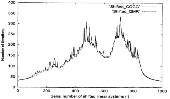
linear systems will remain unsolved by another choice.

Figure 1 shows the number of iterations of each method to solve $Pth$ shifted linear

systems. For example, in Fig. 1, the number of iterations for the shifted COCG method

at $P=600$_{is 150, which}

means

_theshifted

_COCG

_{method required 150}

_iterations

_{to obtain}

the (approximate) solutions of 600th shifted linear systems, i.e., $(\sigma_{600}I-H)x^{(600)}=e_{1}$.

Serialnumberof shifted linearsystems (1)

Figure 1: Number of iterations for the shifted COCG method and the shifted QMRSYM

method

versus

serial number of shifted linear systems.

From Fig. 1 we obtain three observations: first, the two methods required almost the

same

number of iterations at each $\ell$; second, in terms of number of iterations, the shifted

QMR-SYM method often converged slightly faster than shifted COCG method. This

phenomenon is closely related to proposition 2, which will be clearer later; third, for each

method the required number ofiterations depends highly

on

theshift parameters $\sigma_{\ell}$

.

This

result may

come

from varying eigenvalues of the coefficient matrices $\sigma pI-H$ since ifwe

choose $\sigma_{\ell}$ close to

singular. Conversely. from the shape of Fig. 1 we may obtain the partial distribution of

eigenvalues of $H$.

One of the residual 2-norm histories for the two methods is given in Fig. 2. From

Fig. 2

we see

that ${\rm Log}_{10}$ of the relative residua12-norm ofthe shifted QMR SYM method

decreases monotonically and at every iteration step the

norm

is less than that of the

shifted

COCG

method. Hence

we can

say that the property (I) of proposition 2 was

experimentally supported by this history.

$o^{c_{i}}Eo|$ コ

$\frac{..\check\geq\Phi\infty}{\propto Q)}$

Figure 2: ${\rm Log}_{10}$ ofrelative residual 2-norms

versus

the number of iterations ofthe shifted

COCG method and the shifted QMR-SYM method for shifted linear systems with $\ell=$

$701$, i. e., $\sigma_{701}=1.100+0.001i$.

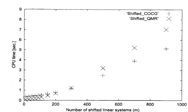
Each computational time of the two methods is given in Fig. 3, where the horizontal

axis denotes the number of shifted linear systems that

are

solved from $\ell=1$ to $m$. For

example, in Fig. 3, the computational time of the shifted COCG method at $m=200$ is

about 0.76 [sec.], which

means

that it required about 0.76 [sec.] to solve theshifted linear

systems: $\{(0.400+0.001i)I-H\}x^{(1)}=e_{1},$ $\{(0.401+0.001i)I-H\}x^{(2)}=e_{1},$ $\ldots,$ $\{(0.599+$

$0.001i)I-H\}x^{(200)}=e_{1}$. From Fig. 3 we

see

that

as

the number $m$ grows larger, the

shifted QMR method required the CPU time

more

than the shifted COCG method.

In Fig. 3

we can

know little about the properties of the two methods for small $\ell$.

Hence,

we

show the ratio of the CPU time of the shifted QMR-SYM method to that

of the shifted COCG method in Fig. 4. We

see

from Fig. 4 that in terms of ratio of

CPU time, theshifted QMR-SYM methodconverged muchfaster than the shifted COCG

method when the number of shifted linear systems is small, say, $m<200$

.

This can be

explained in the following way: for small $m$, updating approximate solutions does not

affect the CPU time

so

much. Other operations such as matrix-vector multiplications

Number ofshifted inear systems (m)

Figure 3: Required CPU timegiven in secondsversus thenumber ofshifted linearsystems for each iterative method.

1.8 1.6 1.4 $=\in\Phi$ 12 $\supset L\circ$ 1 $\ovalbox{\tt\small REJECT}_{08}$ $\frac{.\underline{o}}{\not\subset t0}$ 0.6 0.4 0.2 $0$ $0$ 200 400 600 800 1000

Number of shifted inear systems (m)

Figure 4: The ratio of the CPU time of the shifted QMR-SYM method to that of the

the

same

number of iterations, see Fig. 1. From proposition 2 (I)

we

know that in this

case

the cost of matrix-vector multiplication for the shifted QMR-SYM _method is niuch

cheaper than that for the shifted COCG method since the shifted QMR-SYM method

require real matrix-real vector multiplications and the shifted

COCG

method requires

real matrix-complex vector multiplications. Moreover, dot products and vector additions

of the complex symmetric Lanczos process used in the shifted QMRSYM method

can

be done in $re$al arithmetic. Hence, the shifted QMR-SYM method converged much faster

than the shifted COCG method for

a

small number ofshifts.

4

Concluding remarks

In this paper, with the aim ofsolving cornplex symmetricshifted linear systems efficiently,

we have derived the shifted QMR-SYM method from two important results givenin [2, 3].

The method has

an

advantage

over

the shifted COCG method in that it has

no

need to

choose

a

suitable seed system. From the results of

a

numerical example, we have learned

that for a small number of shifts the shifted QMR SYM method converged much faster

than the shifted COCG method. In this case, the shifted QMR-SYM method is

a

method

of choice for solving complex symmetric shifted linear systems arising from electronic

structure theory.

Acknowledgments

We-would like to thank Prof. Takeo Fujiwara (The University ofTokyo) and Prof. Takeo

Hoshi (Tottori University) for providing

us a

test problem used in the numerical

experi-ment.

References

[1] R. W. FREUND, On conjugate gradient type methods and polynomialpreconditioners

for

a class

_of

complex non-Hermitianmatrices, Numer. Math., 57 (1990), pp. 285-312.

[2] R. W. FREUND, Conjugate gradient-type methods

_for

linear systems with complex

symmetric

_coefficient

matrices, SIAM J. Sci. Stat. Comput., 13 (1992), pp. 425-448.

[3] R. W. FREUND, Solution

_{of Shifted}

Linear Systems by Quasi-Minimal Residual

Itemtions, Numerical Linear Algebra, L. Reichel, A. Ruttan and R. S. Varga eds.,

W. de Gruyter, (1993), pp.

101-121.

$[4|$ R. W. FREUND AND N. M. NACHTIGAL, $QMR;$ A quasi-minimal residual method

for

non-Hermitian linear systems, Numer. Math., 60 (1991), pp. 315-339.

[5] A. FROMMER, $BiCGStab(\ell)$

for families of shifted

linear systems, Computing 70

[6] A. FROMMER AND U. GR\"ASSNER, Restarted GMRES

_for

_shifted

linear systems,

SIAM J. Sci. Comput. 19 (1998), pp. 15-26.

[7] G. H. GOLUB AND C. F. VAN LOAN, Matrix computations, 3rd ed., The Johns

Hopkins University Press, Baltimore and London, 1996.

[8] C. LANCZOS, An itemtion method$f_{0^{\backslash }}r$ the solution

of

the eigenvalueproblem

_of

linear

differential

and integml opemtors, J. Res. Nut. Bur. Standards, 45 (1950), pp.

255-282.

[9] V. SIMONCINI, Restarted

_full

orthogonalization method

_{for shifted}

linear systems,

BIT Numerical Mathematics, 43 (2003), pp. 459-466.

[10] V. SIMONCINI AND D.B. SZYLD, Recent computational developments in Krylov

sub-space methods

_for

linear systems, Num. Lin. Alg. with Appl.,

14

(2007), pp.

1-59.

[11] T. SAKURAI AND H. SUGIURA, A projection method

_for

generalized eigenvalue

prob-lems using numerical integration, J. Comput. Appl. Math., 159 (2003), pp. 119-128.

[12] T. SOGABE AND S.-L. ZHANG, $\mathcal{A}$ COCR method

for

solving complex symmetric

linear systems, J. Comput. Appl. Math., 199 (2007), pp. 297-303.

[13] T. SOGABE, T. HOSHI, S.-L. ZHANG, AND T. FUJIWARA, A numerical method

_for

calculating the Green’s

_function

arising

_from

electronic structure theory, in: Frontiers

of Computational Science, eds. Y. Kaneda, H. Kawamura and M. Sasai,

Springer-Verlag, Berlin/Heidelberg, 2007, pp. 189-195.

[14] R. TAKAYAMA, T. HOSHI, T. SOGABE, S.-L. ZHANG, AND T. FUJIWARA, Linear

algebmic calculation

_of

Green’s

_{function for}

large-scale electronic structure theory,

Phys. Rev. $B73$_, 165108 _{(2006), pp.} 1-9.

[15] H. A. VAN DER VORST AND J. B. M. MELISSEN, A Petrov-Galerkin type method

for

solving $Ax=b$, where $A$ is symmetric complex, IEEE Trans. Mag. 26(2) (1990),