TUMSAT-OACIS Repository - Tokyo University of Marine Science and Technology (東京海洋大学)
Experimental study on wave attenuation due to
flexible intertidal vegetation(柔軟な干潟上植
生による波浪減衰に関する実験的研究)
学位名
修士(工学)
学位授与機関
東京海洋大学
学位授与年度
2019
Master’s Thesis
EXPERIMENTAL STUDY ON WAVE ATTENUATION DUE
TO FLEXIABLE INTERTIDAL VEGETATION
March 2020
Graduate School of Marine Science and Technology
Tokyo University of Marine Science and Technology
Master’s Course of Marine Resources and Environment
Master’s Thesis
EXPERIMENTAL STUDY ON WAVE ATTENUATION DUE
TO FLEXIABLE INTERTIDAL VEGETATION
March 2020
Graduate School of Marine Science and Technology
Tokyo University of Marine Science and Technology
Master’s Course of Marine Resources and Environment
Abstract
Intertidal vegetation grows in the transition region between land and sea, providing habitat for coastal organisms and impacting on coastal ecological structures and food chains. It not only plays an important role in communicating with the land and sea ecosystems, but also can resist and reduce damages due to waves to the shoreline. Another physical effect of intertidal vegetation is it changes transport and diffusion of sediment and marine pollutants along the coast, which depends significantly on velocity distribution inside and outside of vegetation region.
At present, there are many researches on rigid intertidal vegetations. However, the distribution of them is regional and limited, and flexible intertidal vegetation are more widely distributed around the world. Scirpus mariqueter, a native vegetation in China, is also a kind of flexible coastal vegetation which has been greatly reduced due to the biological invasion. It has been strongly supported for conservation and recommended as restoration material of coastal vegetation by the government of China. In the present study, the physical effect of flexible vegetation on wave decay was investigated by using vegetation model in an experimental flume.
The experiment in this paper is divided into two parts. The first part is wave decay measurements on vegetation models for different water depth, vegetation density and vegetation flexibility. The free surface elevation at three wave gauges for every case was measured and the wave decay ratio between at the front of vegetation model and the back of it was calculated. The vegetation model used in the experiment is made by a 3-D printer. In order to find the difference between flexible and rigid vegetation for wave decay, the further experiment was performed. The wave decay ratio was measured for flexible and rigid
vegetation model under the conditions of the same wave, vegetation density and vegetation belt length.
The second part of the experiment is velocity fields measurement on vegetation models for different flexibility by using Particle Image Velocimetry (PIV). Velocity field above the vegetation model was measured when water depth was 16cm, while height of the vegetation models was 12cm. The frame rate for PIV was 1/500s and more than 8000 frames have been captured.
The results of the experiment are shown as follow:
1. Under conditions of the same vegetation density and water depth, wave height decreases along the horizontal distance and significantly decreases in region of vegetation model. 2. Under conditions of the same vegetation density, the decay ratio of wave height
decreases with increase of water depth, showing approximate linear changes. Higher vegetation density gives larger absolute value of the slope of linear functions.
3. Under conditions of the same water depth, wave decay ratio increases with vegetation density. The linear fitting shows that the decay ratio variation with density is larger for the smaller water depth.
4. Both the flexible and rigid vegetation model have some effects on wave decay. When the water depth is smaller than the height of model, decay ratio of rigid model is higher than that of the flexible model. When the water depth exceeds the height of model, the decay ratio of rigid model decreases a lot and is smaller than that of the flexible model under the same water depth.
5. In the case of no vegetation model, the velocity field is very consistent and can be clearly seen that all the velocity vectors are in the same direction. In the cases with rigid and flexible vegetation models, the velocity fields are disturbed by vegetation. Moreover, there are have boundary layers between the canopy region and open water region in both cases of rigid and flexible vegetation, and the boundary layer thickness is thicker in the
rigid vegetation model.
6. At the wave crest phase, the horizontal averaged velocity on flexible vegetation model can be slightly smaller than the case of rigid vegetation which is much smaller than that for the no vegetation model. However, the magnitude of flexible vegetation model is larger at the wave trough phase. The averaged velocity distribution is more variable on the flexible vegetation model both at the wave crest and trough phases, which means flexible vegetation may affect the velocity fields more than the rigid vegetation.
Contents
Abstract ... I
Chapter 1: Introduction ... 1
1.1 Background ... 1
1.2 Motivations and objectives of the study ...4
1.3 Outline of the thesis... 6
Chapter 2: Laboratory experiment of wave decay measurements on vegetation models ... 7
2.1 Introduction ... 7
2.2 Methodology ... 8
2.2.1 Experimental setup and instrumentation ... 8
2.2.2 Vegetation model ... 12
2.2.3 Experimental conditions ... 16
2.2.4 Data processing ... 17
2.3 Results and conclusion ... 18
2.3.1 Wave decay on flexible vegetation models ... 19
2.3.2 Wave decay on different flexibility of vegetation models ... 27
Chapter 3: Laboratory experiment of velocity fields measurement on vegetation models by using Particle Image Velocimetry (PIV) ... 30
3.1 Introduction ... 30
3.2 Principle of Particle Image Velocimetry(PIV) ... 32
3.3 Methodology ... 33
3.3.2 Calibration ... 37
3.3.3 Data processing ... 37
3.4 Results and conclusion ... 40
3.4.1 Velocity fields... 40
3.4.2 Velocity distribution ... 42
Chapter 4: Conclusions and limitations ... 45
References ... 47
Chapter 1: Introduction
1.1 Background
Coastal cities have rich natural resources, convenient transportation and dense population, which are important economic development areas in coastal countries. It is necessary to construct effective measures to protect shorelines and artificial coastal structures to reduce the damage of extreme marine disasters such as tsunami, storm surge and so on. Many traditional coastal engineering measures mainly focus on raising the elevation of seawalls and building submerged breakwaters in front of seawalls (Cheng, 2016). Although they can play effective and stable roles in reducing waves and preventing coastal erosion, their construction and maintenance costs are too high, and they may cut off the original material exchange between land and ocean lives completely, because it is hard for the land organism to get into the ocean through that concrete structures and it is hard too for the ocean organism. These artificial structures may destroy the habitat of intertidal organisms by making ecological imbalance. With the increasing awareness of ecological protection in recent years, coastal protection with using vegetation has become an important development direction of coastal protection.
Intertidal vegetation grows in the transition region between land and sea, providing habitat for coastal organisms and directly impacting on coastal ecological structures by changing the distribution and transportation of dissolved oxygen, inorganic salt and organic nutrition in water. They can not only communicate with the land and sea ecosystems, keep the integrity of food chain and intercept the based-land pollutant, but also can resist and reduce the damage due to waves to the shorelines and coastal structures by their root, stem and leaf, which can produce double benefits in the protection of ecological and physical environment (Yuan, 2013; Cheng, 2018). For example, in the event of the 2004 Indian Ocean tsunami,
areas with coastal tree vegetation were markedly less damaged than areas with no vegetation (Danielsen et al, 2005; Iverson et al, 2007). There is approximately 80% of a 30-year-old
mangrove forest would absorb 50% of the tsunami's hydrodynamic force (Yanagisawa et al,
2010; Wang et al, 2016). Similarly, the vegetated dune at Misawa was the primary factor in tsunami mitigation after the 2011 Great East Japan tsunami, and next are dune only, vegetation only and bare land (Nandasena et al, 2012). Moreover, along the east coast of the United States, damage to shorelines protected by marsh was less than that with artificial facilities following a category 1 hurricane event (Gittman et al, 2014; Hawkins et al, 2019). A 62 million-US-dollar-program has been endorsed to restore and preserve the coastal vegetation in 12 Asian and African countries to against the future tsunamis (Baird, 2006; Wang et al, 2016).
However, rigid intertidal vegetation, such as the mangrove which can reduce waves obviously as mentioned above, are found to be mainly distributed between 5°N and 5°S latitude by using earth observation satellite data. The total area of mangroves in the year 2000 was 137760 km2 in 118 countries and territories in the tropical and subtropical regions of the world. Approximately 75% of world’s mangroves are found in just 15 countries (Giri, 2011). Therefore, for most temperate coastal countries, it is not suitable to grow such rigid intertidal vegetation. Instead, flexible intertidal vegetations are more widely distributed around the world.
On the other hand, the vegetation selected for research in this paper is Scirpus mariqueter, a native herbaceous perennial in China, which also a kind of flexible intertidal vegetation that is distributed in the coastal beach of the Yangtze estuary (Ding et al, 2015; Tao et al,2018). In recent years, the Chinese government has carried out many researches and projects to try to support for conservation and recommended as restoration material of coastal vegetation because it has been greatly reduced due to biological invasion. In April 2016, the government began the program of ecological restoration and reconstruction of Scirpus mariqueter community in Shanghai (Tao et al,2018). The restoration effect of this project is remarkable,
and the species and quantity of aquatic vegetations and animals are obviously increased, which brings a positive effect to the ecological stability. The propagate coefficient of vegetation was high and covered well (see Figure 1.1.1). Meanwhile, the central government of China issued a document on the use and protection of the coast in 2017, which specified that at least 35% of its shoreline should be maintained in a natural state by 2020 (Hawkins et al,2019).
Fig.1.1.1 Ecological restoration effect of Scirpus mariqueter in nanhui, Shanghai (Tao et al,2018)
1.2 Motivations and objectives of the study
At present, there have been a lot of researches which focused on rigid vegetation under the action of waves, but because flexible intertidal vegetation can be swung in the waves, its influence on the wave propagation will be very different from that by rigid vegetation. Studies on the wave attenuation characteristics of flexible intertidal vegetation are far from enough, especially on the difference of velocity fields between flexible and rigid vegetation. Therefore, this thesis will do research on these aspects to improve it.
At the same time, Scirpus mariqueter, as an important intertidal vegetation which needs to be restored. The Chinese government has carried out many researches and projects to try to support for conservation. And due to the excessive development of coastal regions in recent years, extensive intertidal wetlands have shrunk, so this study is also important to prevent further decrease of coastal wetlands and maintain the coastal ecological balance.
Based on the above motivations, the main objectives of this study are as follows:
1. Since there are few studies on the wave attenuation due to flexible intertidal vegetation, the first objective of this study is to understand the wave attenuating ability of flexible vegetation, through wave decay measurements on flexible vegetation model under the action of regular waves with changing water depth and vegetation density in the experimental wave flume.
2. The second objective is to better understand the difference of wave attenuation between flexible and rigid intertidal vegetations, through wave decay measurements on flexible and rigid vegetation models under regular waves with changing water depth in the experimental wave flume.
closely related to the transport and diffusion of sediment and marine pollutants along the coast. The velocity distribution of wave action with vegetation is the basis for further study of their vorticity field characteristics, turbulence characteristics and transportation characteristics. Up to now, less attention has been paid to it, especially the difference between flexible and rigid vegetation in this way. Therefore, the third objective of this study is to understand the difference of velocity fields on flexible and rigid vegetation models by using the Particle Image Velocimetry (PIV) technology.
1.3 Outline of the thesis
1. The background of this study will be given in chapter1, including the benefits and cases of using intertidal vegetation to be a material of coastal protection, and the reasons to choose flexible intertidal vegetation in this study.
2. The laboratory experiment of wave decay measurements on vegetation models will be introduced in chapter2. The experiment was designed to measure the wave height and calculate the wave decay ratio due to vegetation models, then compared the difference between flexible and rigid vegetation models.
3. The laboratory experiment of velocity fields measurement on vegetation models by using Particle Image Velocimetry technology will be introduced in chapter3. The experiment was designed to measure the velocity distribution and compared the difference between flexible and rigid vegetation models.
4. The final conclusions of the wave attenuation, velocity fields and averaged velocity distribution will be given at last.
Chapter 2: Laboratory experiment of wave decay measurements
on vegetation models
2.1 Introduction
In this chapter, an experiment of wave decay due to vegetation models in a wave flume is described. The experiment is divided into two groups. The first group is to study the wave attenuation due to flexible vegetation model under the action of regular waves with changing water depth and vegetation density. The second group is to study the difference of wave attenuation between flexible and rigid vegetation models under regular waves with changing water depth.
2.2 Methodology
2.2.1 Experimental setup and instrumentation
The laboratory experiments were carried out in the wave flume in the Coastal Environment and Engineering Laboratory of Tokyo University of Marine Science and Technology. The wave flume was 720cm long, 15cm wide and 30cm high, as shown in Fig.2.2.1 and Fig2.2.2. It was equipped with a computer-controlled piston-type wave-maker at one end (Feng, 2013). The components of wave maker are step motor, slider and wave paddle, which presented in the Fig2.2.3. In order to reduce the wave reflection from the wall of wave flume, the absorbing materials are placed on both ends of wave flume, as shown in Fig.2.2.4.
Fig.2.2.3 Wave generation system of the flume
The type of wave gauge used in the experiment is CHT6-30 and presented in the Fig.2.2.5, which made by KENEK company. The positions of these three wave gauges are shown in Fig.2.2.2, where the distance between ch2 and ch3 is 135.4cm, located in front of the vegetation model and the back of it. The data capture system consists of wave gauge, BNC cable, initial data collector, data box and c-logger software, as shown in Fig.2.2.6.
Fig.2.2.5 Wave gauge used in the experiment
Before the experiment, calibration of the wave gauges was carried out to obtain the relationship between water elevation and output voltage value. Raise the water surface to the appropriate position so that it can be measured by wave gauge from 5cm up to 5cm down. Set the initial water level at 0, then raise it 5 times, each time by 1cm and get the voltage value. Similarly, drop the water level down 5 times, each time by 1cm and get the voltage value. Finally, the regression lines and calibration functions of each wave gauge are obtained in the Fig.2.2.7.
Fig.2.2.7 Calibration data of the wave gauges
2.2.2 Vegetation model
The vegetation model used in the experiment was printed by the L-DEVO company's 3D printer, M2030TP. The 3D printer is presented in the Fig.2.2.8. The construction of the whole vegetation model belt in the experiment is divided into three steps. Firstly, printed out a piece of vegetation models as shown in Fig.2.2.9. The height of each vegetation model was 12.5cm and the width was 0.3cm. Then, seven pieces were glued to a 2mm transparent plastic
plate to be a unit. One unit of vegetation model is presented in the Fig.2.2.10. In the third step, put all units together to obtain the whole vegetation belt used in the experiment, as shown in Fig.2.2.11.
Fig.2.2.8 L-DEVO M2030TP 3D printer
Fig.2.2.10 One unit of vegetation models
Fig.2.2.11 The whole vegetation model belt
In the first group of this experiment, there are three kinds of densities of vegetation models were used, 0ind/m2, 3660ind/m2 and 11025ind/m2. The vegetation model arrangement is
unchanged at 11025 ind/m2, and two kinds of flexibility were printed, flexible and rigid
vegetation model, as shown in the Fig.2.2.13.
Fig.2.2.12 Vegetation model arrangements. (a)No vegetation, (b)Low density, (c)High density
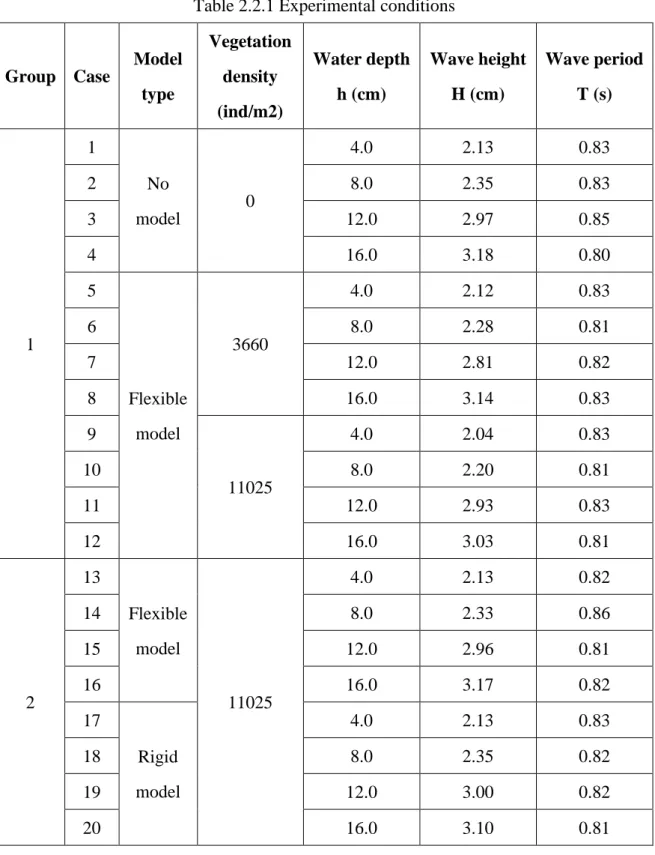
2.2.3 Experimental conditions
The experiment was conducted for twenty cases with different conditions, which divided into the two groups. The conditions were summarized in the Tab.2.2.1.
Table 2.2.1 Experimental conditions
Group Case Model type Vegetation density (ind/m2) Water depth h (cm) Wave height H (cm) Wave period T (s) 1 1 No model 0 4.0 2.13 0.83 2 8.0 2.35 0.83 3 12.0 2.97 0.85 4 16.0 3.18 0.80 5 Flexible model 3660 4.0 2.12 0.83 6 8.0 2.28 0.81 7 12.0 2.81 0.82 8 16.0 3.14 0.83 9 11025 4.0 2.04 0.83 10 8.0 2.20 0.81 11 12.0 2.93 0.83 12 16.0 3.03 0.81 2 13 Flexible model 11025 4.0 2.13 0.82 14 8.0 2.33 0.86 15 12.0 2.96 0.81 16 16.0 3.17 0.82 17 Rigid model 4.0 2.13 0.83 18 8.0 2.35 0.82 19 12.0 3.00 0.82 20 16.0 3.10 0.81
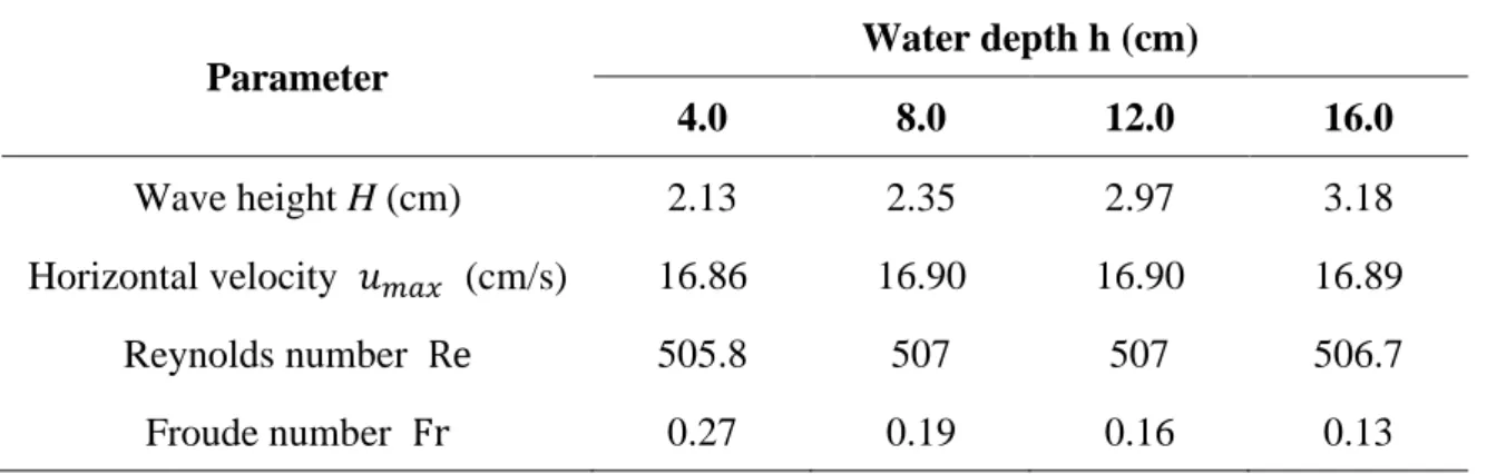
Before investigating the wave attenuation along vegetation model region, the hydrodynamic parameters for different water depths are studied as listed in Tab.2.2.2. Here, 𝑢𝑚𝑎𝑥 is the averaged horizontal velocity at wave crest at different water depth, which measured by PIV. The Reynolds number and Froude number are
𝑅𝑒 = 𝑢max𝑑
ν (2.1)
𝐹𝑟 = 𝑢max
√gℎ (2.2)
Table 2.2.2 Hydrodynamic parameters for different water depth
Parameter Water depth h (cm) 4.0 8.0 12.0 16.0 Wave height H (cm) 2.13 2.35 2.97 3.18 Horizontal velocity 𝑢𝑚𝑎𝑥 (cm/s) 16.86 16.90 16.90 16.89 Reynolds number Re 505.8 507 507 506.7 Froude number Fr 0.27 0.19 0.16 0.13
2.2.4 Data processing
For every case at least 4941 original data were recorded by wave gauges, and the time interval of each data is 0.01s. The calibration data results the form of the calibration equation as follows,
𝑦 = 𝑎𝑥 + 𝑏 (2.3)
Then according to the calibration result to calculate the water surface elevation value, where 𝑥0 is the outputted voltage from the wave gauges.
𝜂0 = 𝑎 ∙ 𝑥0+ 𝑏 (2.4)
𝜂′ = 𝜂0−
∑49411 𝜂0
4941 (2.5)
𝜂𝑅.𝑀.𝑆. = √
∑4941(𝜂′2) 1
4941 (2.6)
Because the waves were assumed to be regular, the wave height 𝐻 is,
𝐻 = 2√2𝜂𝑅.𝑀.𝑆. (2.7)
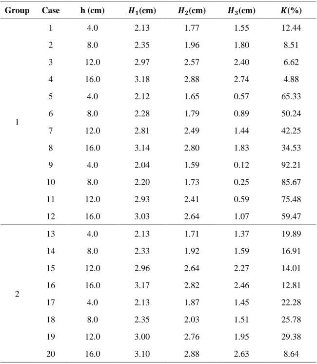
In the experiment of wave attenuation, the wave height decay ratio K is usually taken as the index of wave attenuation degree. The equation is
𝐾 = (1 −𝐻3 𝐻2
) × 100% (2.7)
Where, the value of 𝐻2 is the incoming wave height in front of vegetation models, and the value of 𝐻3 is the wave height after vegetation models. If the wave decay ratio is larger, the attenuation of wave passing through the flexible vegetation belt is more obvious.
2.3 Results and conclusion
Table 2.3.1 The wave height and wave decay ratio of different cases Group Case h (cm) 𝑯𝟏(cm) 𝑯𝟐(cm) 𝑯𝟑(cm) 𝑲(%) 1 1 4.0 2.13 1.77 1.55 12.44 2 8.0 2.35 1.96 1.80 8.51 3 12.0 2.97 2.57 2.40 6.62 4 16.0 3.18 2.88 2.74 4.88 5 4.0 2.12 1.65 0.57 65.33 6 8.0 2.28 1.79 0.89 50.24 7 12.0 2.81 2.49 1.44 42.25 8 16.0 3.14 2.80 1.83 34.53 9 4.0 2.04 1.59 0.12 92.21 10 8.0 2.20 1.73 0.25 85.67 11 12.0 2.93 2.41 0.59 75.48 12 16.0 3.03 2.64 1.07 59.47 2 13 4.0 2.13 1.71 1.37 19.89 14 8.0 2.33 1.92 1.59 16.91 15 12.0 2.96 2.64 2.27 14.01 16 16.0 3.17 2.82 2.46 12.81 17 4.0 2.13 1.87 1.45 22.28 18 8.0 2.35 2.03 1.51 25.78 19 12.0 3.00 2.76 1.95 29.38 20 16.0 3.10 2.88 2.63 8.64
2.3.1 Wave decay on flexible vegetation models
As described above, there are two groups in this experiment. In the first group, a total of three vegetation densities were designed. Fig.2.3.1 to Fig.2.3.4 show snapshots at the experiment for different water depth under the condition of low vegetation model density, and Fig.2.3.5 to Fig.2.3.8 show them for high vegetation model density.
Fig.2.3.1 Snapshot for case5 (h=4.0cm, H=2.12cm)
Fig.2.3.3 Snapshot for case7 (h=12.0cm, H=2.81cm)
Fig.2.3.4 Snapshot for case8 (h=16.0cm, H=3.14cm)
Fig.2.3.6 Snapshot for case10 (h=8.0cm, H=2.20cm)
Fig.2.3.7 Snapshot for case11 (h=12.0cm, H=2.93cm)
Taking the horizontal distance as the abscissa and the wave height as the ordinate, wave height variations along the horizontal distance for group1 cases are presented in the Fig.2.3.9 to Fig.2.3.11. Each of the figure shows results for the same vegetation density. It is observed that wave height decreases along the horizontal distance and significantly decreases in region of the vegetation model.
Fig.2.3.10 The result of wave height along horizontal distance with low vegetation density
Taking the water depth as the abscissa and the wave decay ratio as the ordinate, variations of wave decay ratio for different water depth are shown in Fig.2.3.12. Under conditions of the same vegetation density, the decay ratio decreases with increase of water depth, showing approximate linear changes and higher vegetation density gives larger absolute value of the slope of linear functions.
Taking the square root of vegetation density as the abscissa and the wave decay ratio as the ordinate, variations of wave decay ratio for the same water depth are shown in Fig.2.3.13. Under conditions of the same water depth, wave decay ratio increases with vegetation density. The linear fitting shows that the decay ratio variation with density is larger for the smaller water depth.
2.3.2 Wave decay on different flexibility of vegetation models
In the second group of the experiment, two flexibilities of vegetation models were employed. The snapshots of the experiment are presented in the Fig.2.3.14 and Fig.2.3.15. Meanwhile, the results of the wave height along horizontal distance and the wave decay ratio along water depth and vegetation density are presented in Fig.2.3.16 to Fig.2.3.18.
Fig.2.3.14 Snapshot for flexible vegetation model
Fig.2.3.16 The result of wave height along horizontal distance with flexible vegetation model
Fig.2.3.18 The result of wave decay ratio along water depth
From the above figures, both the flexible and rigid vegetation model have some effects on wave decay. When the water depth is smaller than the height of vegetation models, wave decay ratio of rigid vegetation model is higher than that of the flexible vegetation model; when the water depth exceeds the height of model, the wave decay ratio of rigid decreases a lot and is smaller than that of the flexible vegetation model under the same water depth.
In the case 16 and 20, the reason for these results is when the water depth is larger than rigid vegetation height, the wave attenuation ability will be greatly reduced. The decrease maybe slow or sudden, and the slope of decrease maybe varies according to the different experiment. However, when the water depth is larger than flexible vegetation height, the wave decay will be increased to a stable value or increased first and then decreased. When the flexible vegetation condition is compared to the rigid, the result maybe depend on the flexibility of flexible vegetation and the difference value of flexibility between flexible and rigid, which
requires us to use the same martial to make more different flexibilities of vegetation models to do further experiment.
Chapter 3:
Laboratory
experiment
of
velocity
fields
measurement on vegetation models by using Particle Image
Velocimetry (PIV)
3.1 Introduction
Along the coast, the intertidal vegetation not only reduce the wave height, but also change the transport and diffusion of sediment and marine pollutants, which depends significantly on velocity distribution inside and outside of vegetation region. On the purpose of coastal protection, many experiments and numerical simulations were carried out on the interaction between the surface waves and the emerged array of cylinders (Augustin et al,2009; Irtem et al,2008; Huang et al,2011; Iimura et al,2012; Wu et al,2013). Recently, more attention has been paid to the internal and external flow structure in the interaction of vegetation and ocean waves (Nepf et al,2000; Nepf et al,2007; Nepf et al,2008; Wang et al, 2016). The dense canopies of coastal vegetations can alter the flow field from that of a simple bottom boundary layer and influence the material transports, as well as dissipate the wave energy (Reidenbach et al,2007; Nepf et al,2012; Wang et al, 2016). In this aspect, the effects of the submerged canopies on the flow characteristics, the velocity structure, mass transfer and energy dissipation were studied (Lowe et al,2005; Lowe et al,2007). Moreover, numerical solutions were simulated to obtain the precise flow structure to analyze the effect of the vegetation, which provides another quantitative approach (Cui et al,2008; Ma et al,2013; Wu et al,2013).
Even though, our current knowledge of the wave fields with vegetation is still not enough for coastal protection and environmental protection, especially less attention has been paid to compare flexible and rigid vegetation in flow fields. The fundamental studies for the wave
attenuation and the flow field are still insufficient. Meanwhile, the Particle Image Velocimetry (PIV) has been highly developed in recent two decades and employed in vast experiments (Raffel et al., 2007; Wang et al, 2016). The PIV technique has served to measure the flow structure around a single cylinder (Ozgoren, 2006; Dong et al., 2006; Wang et al, 2016).
Therefore, in the present study, an experiment of velocity fields measurement over flexible and rigid vegetation models by using the Particle Image Velocimetry (PIV) was carried out. Because of the limited time, the experiment was only done at the water depth of 16cm, that is the condition of high tide level.
3.2 Principle of Particle Image Velocimetry (PIV)
Particle Image Velocimetry (PIV) is a kind of velocity measurement technique by non-interferential and indirect way. Its characteristic is beyond the limitations of single point velocimetry (such as LDV), which can record whole velocity fields and provide abundant spatial structure characteristics of the flow field. This kind of technique does not interfere in the flow field except for the scattering of tracer particles to the flow field, so it can accurately and effectively measure the flow field (Qie et al,2014).
The experimental setup of a PIV system typically consists of several subsystem. Normally, tracer particles are added to the flow, a light sheet within the flow is illuminated by laser within a short time. It is assumed that the tracer particles move with local flow velocity. The light scattered by the tracer particles is recorded via a high-speed camera. The output of the digital sensor is transferred to the memory of a computer directly and the sophisticated post-processing is required to calculate the displacement of the particle images between the light pulses. Here, Fig.3.2.1 is an example of PIV system (Raffel et al, 2007; Feng, 2013; Zhu, 2018).
3.3 Methodology
3.3.1 Experimental setup and instrumentation
The wave flume and vegetation models of this experiment are the same as those described in Chapter 2, except for the PIV system, shown in Fig.3.3.1. The PIV system in this experiment consists of laser system (including a laser head, laser transmitter and controlling unit), high-speed camera system (including a high-speed CCD camera) and computer system. The Fig.3.3.2 shows snapshot at the experiment of flexible vegetation models by using PIV system and the Fig.3.3.3 shows the region of observation.
The laser system made by KATO LOKEN was used to illuminate the measuring section and the range of the laser thickness is between 1mm to 5mm, which is shown in Fig.3.3.4. The laser head can adjust the laser direction and the thickness of laser sheet and the laser transmitter can adjust the magnitude of laser. Fig.3.3.5 shows the type of high-speed CCD camera HAS-D72, which was made by DITECT. Its maximum frame rate is 2000 fps with the maximum resolution 1024×1280 pixels. The camera can be trigged and recorded by outer signals (Zhu, 2018).
In addition, PIV is an indirect way to obtain the velocity of particles rather than the velocity of fluid. So, the quality of tracer particles play an important role to the results. The concentration of the tracer particles must be tested to make sure good image can be obtained by adding proper quantity. In this experiment, tracer particles HGS Hollow Glass Spheres produced by DANTEC were used and their diameter is 10μm, as shown in Fig.3.3.6 (Zhu, 2018).
Fig.3.3.1 PIV system
Fig.3.3.3 The region of observation in this experiment
Fig.3.3.5 High-speed CCD camera
3.3.2 Calibration
Before the experiment, the calibration experiment of PIV was carried out to obtain the relationship between the pixel distance and the real distance. A ruler was placed in the middle of wave flume, in the same position of laser sheet, and used the high-speed camera to capture the images, as shown in Fig.3.3.7. Then all frames were inputted to the software named Motion Studio, which can directly transfer the distance unit from pixel to centimeter.
Fig.3.3.7 Calibration
3.3.3 Data processing
For every case at least 8000 original images were recorded by high speed camera, and the time interval of each image is 0.002s. The main idea of the PIV evaluation is based on digital
spatial correlation analysis. Firstly, the particles are illuminated by laser and the second frame is recorded at a short time later during which the particles will have moved according to the flow. The spatial translation of groups of particles can be observed. The image pair can yield a field of linear displacement vectors where each vector is formed by analyzing the movement of localized groups of particles. In practice, this is accomplished by extracting small samples or interrogation windows and analyzing them statically, as shown in Fig.3.3.8 (Feng, 2013; Zhu, 2018).
Fig.3.3.8 Sketch for illustration of interrogation window (Raffel et al, 2007; Feng, 2013; Zhu, 2018)
The method to find the best match between the images in a statistical sense is accomplished by using the discreet cross-correlation function, whose integral function is shown as Eq.3.1:
𝑅𝐼𝐼(𝑥, 𝑦) = ∑ ∑ 𝐼(𝑖, 𝑗)𝐼′(𝑖 + 𝑥, 𝑗 + 𝑦) 𝐿 𝑗=−𝐿 𝐾 𝑖=−𝐾 (3.1)
The variable I and I’ are the samples as extracted from the images where I’ is larger than the template I. Especially, the template I is linearly shifted around in the sample I’ without extending over edges of I’. For each choice of sample shift (x,y), the sum of the products of all overlapping pixel intensities produces one cross-correlation value RII(x,y). By applying
this operation for a range of shifts (−M ≤ x ≤ +M, −N ≤ y ≤ +N), a correlation planes the size of (2M+1) × (2N+1) is formed. This is shown in Fig.3.3.9. For shift values at which the samples particle images align with each other, the sum of the products of the pixel intensities will be larger than elsewhere, resulting in a high cross-correlation value RII at this position.
Especially, the cross-correlation function statistically measures the degree of match between the two samples for a given shift. The highest value in the correlation plan can then be used as d direct estimate of the particle image displacement (Feng, 2013; Zhu, 2018).
Fig.3.3.9 Sketch of the illustration of the direct cross correlation (Raffel et al, 2007; Feng, 2013; Zhu, 2018)
For several cases it may be useful to quantify the degree of correlation between the two image samples. The standard cross-correlation function Eq.3.2 will yield different maximum correlation values for the same degree of matching because the function is not normalized. For instance, samples with many (or brighter) particle images will produce much higher
correlation values than interrogation windows with fewer (or weaker) particle images. This makes a comparison of the degree of correlation between the individual interrogation windows impossible. The correlation coefficient function normalizes the cross-correlation function Eq.3.2 properly:
c𝐼𝐼(x, y) = c𝐼𝐼(x, y) √𝜎𝐼(𝑥, 𝑦)√𝜎𝐼′(𝑥, 𝑦) (3.2) where c𝐼𝐼(x, y) = ∑ ∑[𝐼(𝑖. 𝑗) − 𝜇𝑖] 𝑁 𝑗=0 𝑀 𝑖=0 [I′(i + x, j + y) − μI′(x,y)] (3.3) 𝜎𝐼(𝑥, 𝑦) = ∑ ∑[𝐼(𝑖. 𝑗) − 𝜇𝐼]2 𝑁 𝑗=0 𝑀 𝑖=0 (3.4) 𝜎′ 𝐼(𝑥, 𝑦) = ∑ ∑[𝐼′(𝑖.𝑗)− 𝜇𝐼′(x,y)] 2 𝑁 𝑗=0 𝑀 𝑖=0 (3.5)
The value μi is the average of the template and is computed only once while μi (x, y) is the
average of I’ coincident with the template I at position (x, y). It must be computed for every position (x, y).
3.4 Results and conclusion
3.4.1 Velocity fields
The instantaneous flow fields may be different under the different conditions of vegetation models. Therefore, in this experiment, the velocity fields will be compared with no
vegetation model, rigid vegetation model and flexible vegetation model, as shown in Fig.3.4.1 to Fig.3.4.3.
Fig.3.4.1 The result of instantaneous velocity fields with no vegetation model
In the Fig.3.4.1, when at time a, the water surface is in the trough position. The velocity direction is horizontal to the left and the distribution is very uniform and consistent. When at time b, the water surface began to rise. The velocity direction is slightly to the upper left and the distribution is very uniform and consistent. When at time c, the water surface continues to rise, and the velocity direction is mostly to the upper left, especially near the water surface. When at time d, the velocity direction is mostly to the upward. When at time e, the water surface is about to the crest position. The velocity direction is to the upper right and the distribution is very uniform and consistent. When at time f, the water surface is in the crest position. The velocity direction is horizontal to the right and the distribution is very uniform and consistent. When at time g, the water surface began to down. The velocity
direction is to the lower right and the distribution is very uniform and consistent. When at time h, the water surface continues to down, and the velocity direction is mostly to the downward. When at time i, the velocity direction is mostly to the lower left, especially near the water surface. When at time j, the water surface is about to the trough position, and the velocity direction is slightly to the lower left, especially near the water surface.
From the above results, it can be clearly seen all the velocity vectors are mostly in the same direction in every phase, which means the instantaneous velocity fields in this case are very consistent and stable.
In the Fig.3.4.2, when at time a, the water surface is in the trough position. The velocity direction is horizontal to the left and has the boundary layer between the vegetation canopy and open water region. When at time b, the water surface began to rise. The velocity direction is slightly to the upper left and is to the downward near the vegetation canopy. When at time c, the water surface continues to rise, and the velocity direction is mostly to the upper left and it also has the boundary layer between the vegetation canopy and open water region. When at time d, the velocity direction is mostly to the upward and it has some turbulence and vortex flow. When at time e, the water surface is about to the crest position. The velocity direction is to the upper right, right and upper right from left to right region. When at time f, the water surface is in the crest position. The velocity direction is horizontal to the right and the distribution is mostly consistent. When at time g, the water surface began to down, the velocity direction is mostly to the lower right. When at time h, the water surface continues to down, and the velocity direction is mostly to the downward. When at time i, the velocity direction is mostly to the lower left and is to the downward near the vegetation canopy. When at time j, the water surface is about to the trough position, and the velocity direction is slightly to the lower left and it also has the boundary layer between the vegetation canopy and open water region.
From the above results, the velocity vectors are not in the same direction, which means the instantaneous velocity fields are disturbed by vegetation model and the boundary layer between the vegetation canopy region and open water region is very clear.
Fig.3.4.3 The result of instantaneous velocity fields with flexible vegetation model
In the Fig.3.4.3, when at time a, the water surface is in the trough position and the vegetation model moves to the left to the maximum. The velocity direction is horizontal to the left and has the boundary layer between the vegetation canopy and open water region. When at time b, the water surface began to rise. The velocity direction is slightly to the upper left and it also has the boundary layer between the vegetation canopy and open water region. When at time c, the water surface continues to rise, and the velocity direction is mostly to the upper left and it also has the boundary layer. When at time d, the velocity direction is mostly to the upward and has some turbulence and vortex flow. When at time e, the water surface is about
to the crest position. The velocity direction is mostly to the upper right in the open water region and is to the upward above the vegetation canopy. When at time f, the water surface is in the crest position and the vegetation model moves to the right to the maximum. The velocity direction is horizontal to the right in the open water region. In the region above the vegetation canopy, the velocity direction is to the upper right and has the vortex flow. When at time g, the water surface began to down, the velocity direction is mostly to the lower right and it also has the vortex flow. When at time h, the water surface continues to down. The velocity direction is mostly to the lower left in the open water region and is to the downward above the vegetation canopy and it also has some turbulence and vortex flow. When at time i, the velocity direction is mostly to the lower left and is to the downward near the vegetation canopy. When at time j, the water surface is about to the trough position. The velocity direction is slightly to the lower left and is to the downward near the vegetation canopy.
From the above results, the flexible vegetation model moves around every time. The instantaneous velocity fields are variable and disturbed by vegetation model very much. Compared with the rigid vegetation, the boundary layer thickness in flexible is thinner at the wave trough phase, and the size and range of velocity fields variation in flexible is larger at the wave crest phase.
3.4.2 Velocity distribution
From the above results, it is found that the velocity fields at the wave crest and trough are very different. Therefore, the averaged velocity distribution at the two phases are further analyzed and presented in Fig.3.4.4 and Fig.3.4.5.
Fig.3.4.4 The result of averaged velocity distribution at wave crest phase
In the Fig.3.4.4, under the condition of no vegetation model, the velocity ranges from 14 to 17cm/s and decreases very slowly from the bottom to the top. Under the condition of rigid vegetation model, the velocity ranges from 10 to 14cm/s and the velocity distribution process is increases first and then decreases slowly from the vegetation canopy to the top. Under the condition of flexible vegetation model, the velocity ranges from 0 to 14cm/s and the velocity distribution process is increases first and then decreases suddenly from the vegetation canopy to the top.
In the Fig.3.4.5, under the condition of no vegetation model, the velocity ranges from 8 to 12cm/s and increases slowly from the bottom to the top. Under the condition of rigid vegetation model, the velocity ranges from 0 to 14cm/s and the velocity distribution process is slow increases first, sudden increases and then slow increases from the vegetation canopy to the top. Under the condition of flexible vegetation model, the velocity ranges from 0 to 18cm/s and the velocity distribution process is the same as the condition of rigid vegetation model.
The above results show that the horizontal averaged velocity on flexible vegetation model can be slightly smaller than the case of rigid vegetation model which is much smaller than that for no vegetation model at wave crest. However, the magnitude of it is larger than rigid vegetation model at wave trough. The variation of averaged velocity distribution is large on the flexible vegetation model both at the wave crest and wave trough, which means flexible vegetation may affect the velocity fields more than the rigid vegetation.
Chapter 4: Conclusions and limitations
The conclusions can be drawn as follows:
1. Under conditions of the same vegetation density and water depth, wave height decreases along the horizontal distance and significantly decreases in region of vegetation model. 2. Under conditions of the same vegetation density, the decay ratio of wave height
decreases with increase of water depth, showing approximate linear changes. Higher vegetation density gives larger absolute value of the slope of linear functions.
3. Under conditions of the same water depth, wave decay ratio increases with vegetation density. The linear fitting shows that the decay ratio variation with density is larger for the smaller water depth.
4. Both the flexible and rigid vegetation model have some effects on wave decay. When the water depth is smaller than the height of model, decay ratio of rigid model is higher than that of the flexible model. When the water depth exceeds the height of model, the decay ratio of rigid model decreases a lot and is smaller than that of the flexible model under the same water depth.
5. In the case of no vegetation model, the velocity field is very consistent and can be clearly seen that all the velocity vectors are in the same direction. In the cases with rigid and flexible vegetation models, the velocity fields are disturbed by vegetation. Moreover, there are have boundary layers between the canopy region and open water region in both cases of rigid and flexible vegetation, and the boundary layer thickness is thicker in the rigid vegetation model.
6. At the wave crest phase, the horizontal averaged velocity on flexible vegetation model can be slightly smaller than the case of rigid vegetation which is much smaller than that for the no vegetation model. However, the magnitude of flexible vegetation model is larger at the wave trough phase. The averaged velocity distribution is more variable on the flexible vegetation model both at the wave crest and trough phases, which means
flexible vegetation may affect the velocity fields more than the rigid vegetation. While doing experiments the limitations are as follows:
1. Since the printing time of the vegetation model is too long, the rigid vegetation model is only made of short length. It should be better if we provided more vegetation model. 2. The flexible vegetation model used in the experiments is white, but it would have been
References
Augustin L N, Irish J L, Lynett P. Laboratory and numerical studies of wave damping by emergent and near-emergent wetland vegetation[J]. Coastal Engineering, 2008, 56(3).
Baird A H. False hopes and natural disasters. New York Times, 2006.
Cheng J G. Research on dynamic characteristics of wave hydrodynamics in flexible Plant[D]. Changsha University of Science and Technology, 2016.
Cheng M, Liu S G, Lou X, Li X L. Impact of rigid vegetation on wave attenuation and flow structure[J]. Advances in Science and Technology of Water Resources, 2018, 38(06): 32-37.
Cui J, Neary V S. LES study of turbulent flows with submerged vegetation[J]. Journal of Hydraulic Research, 2008, 46(3): 307-316.
Danielsen F, Srensen M K, Olwig M F, Selvam V, Parish F, Burgess N D, Hiraishi T, Karunagaran V M, Rasmussen M S, Hanse L B, Quarto A, Suryadiputra N. The Asian tsunami: a protective role for coastal vegetation[J]. Science, 2005, 310(5748): 643.
Ding W H, Jiang J Y, Li X Z, Huang X, Li X Z, Zhou Y X, Tang C D. Spatial distribution and influencing factors of salt marsh vegetation in the south of dongtan, Chongming[J]. Chinese Journal of Plant Ecology, 2015, 39(07): 704-716.
Dong S, Karniadakis G E, Ekmekci A, Rockwell D. A combined direct numerical simulation- particle image velocimetry study of the turbulent near wake[J]. Journal of Fluid Mechanics, 2006, 569: 185-207.
Feng D J.Laboratory study of bottom boundary layer in the bore-driven swash zone on impermeable slope[D]. Tokyo University of Marine Science and Technology, 2013.
Giri1 C, Ochieng E, Tieszen L L, Zhu Z, Singh A, Loveland T, Masek J, Duke N. Status and distribution of mangrove forests of the world using earth observation satellite data[J]. Global Ecology and Biogeography, 2011, 20: 154-159.
Gittman R K, Popowich A M, Bruno J F, Peterson C H. Marshes with and without sills protect estuarine shorelines from erosion better than bulkheads during a Category 1 hurricane[J]. Ocean and Coastal Management, 2014, 102.
Hawkins S T, Allcock A L, Bates A B, Firth L B, Smith I P, Swearer S E, Todd P A. Design Options, Implementation Issues and Evaluating Success of Ecologically Engineered Shorelines. Oceanography and Marine Biology: An Annual Review, 2019, 57: 169– 228.
Huang Z H, Yao Y, Sim S Y, Yao Y. Interaction of solitary waves with emergent, rigid vegetation[J]. Ocean Engineering, 2011, 38(10).
Irtem E, Gedik N, Kabdasli M S, Yasa N E. Coastal forest effects on tsunami run-up heights[J]. Ocean Engineering, 2008, 36(3).
Iimura K, Tanaka N. Numerical simulation estimating effects of tree density distribution in coastal forest on tsunami mitigation[J]. Ocean Engineering, 2012, 54.
Iverson L R, Prasad A M. Using landscape analysis to assess and model tsunami damage in Aceh province, Sumatra[J]. Landscape Ecology, 2007, 22(3).
Lowe R J, Koseff J R, Monismith S G. Oscillatory flow through submerged canopies: 1. Velocity structure[J]. Journal of Geophysical research oceans, 2005, 110(C10).
Lowe R J, Falter J L, Koseff J R, Monismith S G, Atkinson M J. Spectral wave flow attenuation within submerged canopies: Implications for wave energy dissipation[J]. Journal of Geophysical research oceans, 2007, 112(C5).
Ma G F, Kirby J T, Su S F, Figlus J, Shi F Y. Numerical study of turbulence and wave damping induced by vegetation canopies[J]. Coastal Engineering, 2013, 80.
Nandasena N A K, Sasaki Y, Tanaka N. Modeling field observations of the 2011 Great East Japan tsunami Efficacy of artificial and natural structures on tsunami mitigation[J]. Coastal Engineering, 2012, 67: 1-13.
Nepf H, Vivoni E R. Flow structure in depth-limited, vegetated flow[J]. Journal of Geophysical research oceans, 2000, 105(C12): 28509-28861.
Nepf H, Ghisalberti M, White B, Murphy E. Retention time and dispersion associated with submerged aquatic canopies[J]. Water Resources Research, 2007, 43(4).
Nepf H, Ghisalberti M. Flow and transport in channels with submerged vegetation[J]. Acta Geophysica, 2008, 56(3).
Nepf H. Flow and Transport in Regions with Aquatic Vegetation. Annual Review of Fluid Mechanics, 2012, 44: 123-124.
Ozgoren M. Flow structure in the downstream of square and circular cylinders[J]. Flow Measurement and Instrumentation, 2005, 17(4).
Qie L W; Du C; Zhang X; Jiang X L. Research on the characteristics of the vortex field around breakwaters by the PIV technique[J]. Marine Science Bulletin, 2014, 33(02): 204-214.
Raffel M, Willert C E, Wereley S T, Kompenhans J. Particle Image Velocimetry: A Practical Guide[M]. Springer, 2007.
Reidenbach M A, Koseff J R, Monismith S G. Laboratory experiments of fine-scale mixing and mass transport within a coral canopy[J]. Physics of Fluids, 2007, 19(7).
Tao Y D, Zhong S C, Li C W, Zhao M, Ding P Z, Fang S B, He P M, Yu K F. A study on the effect of ecological restoration and reconstruction of Scirpus mariqueter community: a case of Nanhui coasts[J]. Transactions of Oceanology and Limnology, 2018(05): 40-49.
Wang Q, Guo X Y, Wang B L, Fang Y L, Liu H. 2016. Experimental Measurements of Solitary Wave Attenuation Over Shallow and Intermediate Submerged Canopy[J]. China Ocean Engineering, 2016, 30(03): 375-392.
Wu W, Zhang M L, Yavuz O, Daniel W. Analysis of Vegetation Effect on Waves Using a Vertical 2D RANS Model[J]. Journal of Coastal Research, 2013, 29(2).
Yanagisawa H, Koshimura S, Miyagi T, Imamura F. Tsunami damage reduction performance of a mangrove forest in Banda Aceh, Indonesia inferred from field data and a numerical model[J]. Journal of Geophysical Research Oceans, 2010, 115(6).
Yuan D L. Experiments of flow and suspended sediment in tidal vegetation[D]. East China Normal University, 2013.
Zhu H J. Flow visualization around small roughness elements with a hydraulic scale-up model based on re-fr similarity law[D]. 2018.
Acknowledgment
Two years master study will be finished soon. I really appreciated to all of people who I met in Japan. We have shared two years together and I feel terrible to be apart from them.
I would like to thank my supervisor, Professor Akio Okayasu, for his guidance and suggestions on my study and Japanese life. I always cherish the time spent with him in laboratory and I always like his teaching way in class. To help me get a high quality of paper, he paid a lot of time and energy. I want to express my sincere thanks for his patient and help.
I would like to thank Professor Tsuyoshi Ikeya who had provided me lots of suggestions in my experiment and taught me how to deal with problems. Acknowledgement also to Professor Kazuo Tani, and Associate Professor Daisuke Inazu for their advices in my study.
Furthermore, I want to thank Doctor Feng Dejun for his help in the experimental setup of PIV, which I knew nothing about it at the beginning.
Many thanks are given to all of members in Coastal Environment and Engineering Laboratory including those who have graduated during these two years. Acknowledgement greet to Mr. Yoshiyuki Uno, Mr. Kitamura Fukutaro, Mr. Wang Yulong, Mr. Chen Tianning, Mr. Nguyen Van Khanh, Mr. Luu Trong Hieu, Ms. Moe Yu Par Zaw, Mr. Zhu Haijun, Mr. Yuya Osaki, Ms. Bi Dongxu, Mr. Dobashi Yoichiro (my tutor who helped me adapt to Japanese life), Mr. Yoneyama Yuichi, Mr. Hayashi Fumiyasu, Mr. Orita Kiyotaka.