An Application of Machine Learning Techniques to Plastic Identification Based on Raman Spectroscopy in Industrial Recycling.

(1)

博士学位論文

An Application of Machine Learning Techniques

to Plastic Identification Based on Raman Spectroscopy

in Industrial Recycling

近

畿

大

学

大

学

院

産業理工学研究科産業理工学専攻

(2)

Love to:

Christiany Juditha

Zean Amadeus Marcelino WM Jr.

The fear of the Lord

is the beginning of knowledge

(3)

Preface

Praise and gratitude to God that have given experience, knowledge, and health even all things needed from the beginning of my study until complete the doctoral thesis writing. Hopefully all of what I have done, it can be beneficial for the development science and knowledge especially in plastics recycling industry.

I realized that the results of this work were not yet perfectly, but I have worked optimally to do my best. Therefore, in this moment I would like to say gratefulness for them who support me:

1. My wife Chirstiany Juditha and my son Zean Amadeus Marcelino that have given me spirit by their love and pray.

2. My father Lewi Lembak Musu, my mother Dorkas Sipi Nari Paginta, my sisters and brother, and whole of my family that always pray for me.

3. My supervisors Prof. Hirohumi KAWAZUMI, Prof. Nabuto OKA, and Prof. Mitsuhiko FUJIO that have taught and guided me to get the wealthy science and knowledge. Thank you very much for the generosity and the patience.

4. Dean, Lecturers, and Administration staff in Kindai University, Fukuoka campus. Thank you very much for whole of the hospitality.

5. Yasuo Tsuchida is the president of Saimu Corporation and Akihiro Tsuchida is my co-worker in this study. Thank you very much for the good cooperation during work this research.

(4)

6. Dr. Y. Johny W. Soetikno, SE., MM,the chairman of STMIK Dipanegara Makassar and all my colleague that always support me.

7. All my friends in Aida, Shimizudani-Ryugakusei. Thank you for whole of experience during struggle to achieve our dream.

May God give abundance of blessings in whole of our lives.

Iizuka-Fukuoka, February 2020

(5)

Figures

Number Description Page

2.1 An energy level diagram illustrating the transitions occurring during

Rayleigh scattering and Stokes, and anti-Stokes. ……… 17

2.2 a) Raman spectrum of wet PET bottle. b) Identification of similar type of plastics. ………. 18

2.3 a) Identification of bromine compounds on PP. b) Identification of black plastic. ……… 18

2.4 Raman spectra of polysulfide (red) and polyethylene (green). ……… 20

2.5 Raman spectra of styrene polymers: acrylonitrile butadiene styrene (ABS), styrene-butadiene (SB), polystyrene (PS), and styrene acrylonitrile (SAN). ……… 20

2.6 The illustration of Machine Learning understanding. ……….. 21

2.7 The concept of a unit vector. ……….. 23

2.8 The structure of PCA model. ……… 24

2.9 The illustration of SVM, a) plot of dataset red and blue classes, b) the optimum hyperplane with maximum margin between support vector. ………. 25

2.10 The illustration of ANN concept, a) the biological brain neural networks structure, b) the simulate of biological brain to ANN algorithm. …..………. 29

2.11 Architecture of artificial neural networks. ……….. 30

2.12 The percentages of application statuses of unsupervised learning technique in dimensionality reduction, outlier detection, process monitoring, and data visualization. ……… 33

(8)

2.13 The percentages of supervised learning techniques which is

implementing in industry to handle process monitoring, fault

classification, soft sensor, and quality prediction. ………. 34

3.1 The experimental schema of plastic identification. ……… 37

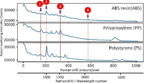
3.2 Essential peaks selection in ABS, PP, and PS spectra. ……….. 37

3.3 Illustration of baseline reduction. ……… 38

3.4 The signal triggered by Gaussian distribution. ……… 40

3.5 The Raman spectra of Polystyrene (PS), original and after adding noise. ……… 41

4.1 The plotting of SVM classification from P1 and P2 peaks pair. …….. 47

4.7 SVM classification of the data with 7.5-times noise addition in similar models. ……… 51

4.8 SVM classification of the data with 15-times noise addition in similar models. ………. 51

4.9 Correlation of the accuracy ratio and the margin value in the SVM classification. ………. 55

4.10 The percentages contribution of correlated information to principal components. ……… 59

4.11 The percentages contribution to Principal Component, a) The contribution to PC1, b) The contribution to PC2. ………... 60

(9)

4.13 The plotting of PCA-SVM classification with data that adding noise

0.75-times. ……….. 61

1.5-times. ……… 62

2.5-times. ………. 63

3.75-times. ……….. 63

7.5-times. ……… 64

15-times. ……….. 65

4.19 The accuracy of 5 times experimental on PCA-SVM technique. …… 66 4.20 Comparison of accuracy between PCA-SVM and SVM. …..………. 67 4.21 Design implementation of machine learning techniques to plastic

Identification in industrial recycling. ………. 72

5.1 Architecture of ANNs classification. ………. 75

5.2 The converging curves of loss value between two and three hidden

layers. ……… 75

5.3 The converging curves of accuracy between two and three hidden

(10)

Tables

Number Description Page

4.1 The maximum margin between support vector in each peak pair. …. 56

4.2 The number of support vector in each peak pair. ……… 56

4.3 Summary of analyzing the categorization correctness based on

Information in Figs. 4.1-4.8. ……….. 57

4.4 Validation accuracy of PCA-SVM and SVM. ………. 70

(11)

Chapter 1 Introduction

The enhancement of plastics utilization grows twenty-fold in period 1964 until 2014, even the prediction will become double in 2050. It means the escalation of plastics production very fast which is in 1964 only 15 metric tons (mt) increased becoming 311 mt in 2014 [1]. The big problem of the condition is it will create imbalance of ecosystem even will make damage of environmental. Indeed, the plastics bring some benefit for human life which caused by characteristic of plastics that low cost, versatile, durable, and high strength-to-weight ratio, yet the handlers of after-use not equal with the quantity of production that cause plastics waste will be collected on

the mainland and in ocean as pollution and can increase CO2 emission which will affect

to global warming.

In World Economy Forum on January 2016 Ellen MacArthur Foundation [2] talk about The New Plastics Economy: Rethinking the Future of Plastics, which explained that global flows of plastic packaging materials in 2013, 98% raw material came from virgin fossil feedstock to produce 78 mt plastic packaging. After usage of the product 40% wasted to landfilled, 32% leakage, 14% to incineration and/or energy recovery, and 14% collected for recycling, wherein 4% will be loss on the processing, 8% recycled for lower-value applications, and only 2% which recycled becoming similar-quality applications by closed-loop recycling method. In addition, 50.1% production of plastics material volume and 82% plastics leaked into the oceans [3]

(12)

occur in Asia. Therefore, to prevent the big risk of environmental damage, further explained that never become plastics as waste after-use, must reduce the leakage of plastics into natural systems drastically, and uncouple plastics from fossil feedstock by improved plastics recycling system radically.

The important purpose of plastics recycle is to reduce emission of carbon dioxide to prevent the global warming effect. From the viewpoint, the basis of plastics recycling method is selected by the advantage of economic opportunities and the aims of recycling product. There are three plastics recycling methods commonly, i.e. mechanical recycling (closed loop recycling), chemical recycling (feedstock recycling)

and thermal recycling (energy recovery).

Mechanical recycling is a way to recycle the plastics waste into new material without changing the basic structure of material before [4]. This process through several step which final product is in pellet shape that will become raw material for textiles, sheeting, injection molding, bottle, etc. Improvement sorting technology are important thinks in mechanical recycling to maintain the purity of material to get higher-value application.

Chemical recycling is a method which used to decompose polymers into monomers component, where the monomers product use as feedstock for new plastics product [5]. The common technology used for decomposition are chemical depolymerization, degradation in microwave reactor, gasification, etc. This method can use as complementary of mechanical recycling when the purify is difficult.

(13)

Thermal recycling or energy recovery is a pathway to use plastics waste as source of energy [6]. By incinerator mechanisms i.e. stoker incinerator, fluidized-bed incinerator, and gasification melting furnace, the heat and exhaust gas generated can be used as new sources of energy in Japan. More than 65% of waste incineration facility in Japan utilize energy from this process. Instead, the slug as residue of processing can also be used as a raw material for others manufacture such as cement.

According H. Ritchie and M. Roser, in Our World In Data 2019[7], the three largest populations of countries in Asia (China, India and Indonesia) is the countries that inadequately managed of plastics waste, where the percentage of mismanaged are 78%, 85%, and 81% respectively, even China and Indonesia are the largest countries which contribute the plastics waste enter into the ocean [3]. Aside from regulation each county, this phenomenon describe that still have big gap between production and utilization with post-use handling of plastics which will bring environmental damage in global scale. It required innovation technology of plastics waste handlers faster.

The objective of this study is to improve the technology of mechanical recycling at the sorting part use Raman spectroscopy as optical apparatus detection, and machine learning technique as intelligent classification algorithm. The advantages our approaches are characteristic of Raman scattering will be sharper & better resolved peaks while and training process in machine learning suitable with industrial atmosphere which can handle changing conditions of raw material without spectroscopic knowledgements.

(14)

The outcome is to get plastic identification method with high level purity in closed-loop mechanism which is implemented on plastics recycling industry scale. And, our new machine learning approach in the plastic classification provide a smart and versatile technique to the on-site identification in actual recycling factory. This study divided into two parts of the study; “Demonstration of Support Vector Machine (SVM) for Selection of Useful Peaks in Raman Spectra” and “Application of Machine Learning Techniques of Principal Component Analysis (PCA) - SVM Combination and Artificial Neural Network (ANN) for Plastic Identification Based on Raman spectroscopy”. The objects of all study using three type of plastic; Polypropylene (PP), Polystyrene (PS), and Acrylonitrile-butadiene-styrene (ABS). They are real waste plastics produced in recycling processes of home appliances industry.

1.1 Demonstration of SVM for Selection of Useful Peaks in Raman Spectra The study of Plastic Identification using Support Vector Machine (SVM) Technique based on Raman spectroscopy is a research to analyze the good peaks combination from Raman spectra when detection the plastic material. As the Raman detection the material will produce spectra which have many peaks in wavelength range 0 – 1300 cm-1. To make faster identification is selected four essential peaks of the spectra that will be figure out the type of material.

Peaks extraction is the next process to get value of each peak as a feature value. There are two processes in this stage i.e. background reduction and calculate peak area. After peaks extraction was obtained dataset with four feature which derive from four

(15)

selected peaks. From the dataset which has been through data normalization yielded six peak combinations which will analyze using SVM to gain the best peak combination to identify the type of plastic. The technique will demonstrate useful selection peaks in Raman spectra. Overall of this study getting two peaks of many peaks in Raman spectra to identify the type of plastic.

1.2 Application of Machine Learning Techniques of PCA - SVM Combination and ANN for Plastic Identification Based on Raman spectroscopy

The aim of this study is to improve the first study with other technique to get robustness identification which will implement in real industrial field. This study uses same dataset with previous study where the dataset has been through data preparation, but in this study utilize entire feature of dataset. The goal of this technique that all of information that contained in four essential peaks used in identification process.

The collection of information from essential peaks use Principal Component Analysis (PCA) by reducing dimension to obtain new dataset with all important information from dimension that eliminated. Further, identification process is applied SVM analysis by optimum hyperplane that will classify the type of plastic. Adding several intensities of noise into original dataset and comparison with others technique done to evaluate the robustness of hyperplane in the classification system.

We also have applied ANN to the categorization of plastics by using all four peaks in the Raman spectra. It is approach could be useful for the requirement of many

(16)

kinds of plastic identification that would be too complicate to categorize them in the two component plots.

1.3 The systematic of Writing

To achieve systemic exposure, the writing is as follows:

a) Chapter 1: Explanation about phenomenon, problem, objective, and scope of this research.

b) Chapter 2: The theoretical basis and literature which became research underlying. c) Chapter 3: Explanation about experimental stages of plastic identification using

Raman spectroscopy which starts from data preparation, method implementation, and measurement.

d) Chapter 4: Explanation about quantitative evaluation for the peak selection in the Raman spectroscopy classification of plastics based on the Support Vector Machine and plastic identification using PCA-SVM for industrial field.

e) Chapter 5: Describing about plastic classification using ANN technique. f) Chapter 6: Conclusion of this research and suggestion for implementation.

(17)

Chapter 2 Literature Review and Theoretical Framework

This chapter is collection of interrelated concepts, theory and previous research that already exist which underlie all of explanation in this study. It will describe reason and boundary of research problem base on the result of studies before and will give frame to solve the problem.

2.1 Roadmap of previous researches

In this section will explain the previous research around plastic solid waste (PSW) problem, impact for human life and environmental of PSW problem, the effort which has done to prevent the global environmental damage, and the technology development to cover out the problem. The previous research is the basic and as a starting point of this study.

2.1.1 Plastic waste

According Masaru Tanaka in Municipal Solid Waste Management in Asia and the Pacific Islands, 2014 [8]., that nowadays, there are three major environmental crisis which are tightly related with waste and waste management i.e., global warming crisis, resource crisis, and ecosystem crisis. The Global warming crisis due to increasing of greenhouse gas emissions encompass carbon dioxide which will escalate

the global temperature up to 6.4 O_{C in the twenty-first century. It caused of waste}

incineration that emits carbon dioxide and landfilling generates which produce greenhouse gases such as methane. Resource crisis in consequence of global society

(18)

have consumed unlimited natural resources in the past that cause mineral resources are predicted will exhaust in 30-40 years later. The emphasis of resource conservation is recycling. Ecosystem crisis caused by mistake of waste management that has an impact to soil erosion, water deficiency, water contamination, and air pollution. It should be tackled with stop to open landfill dumping and the open burning waste.

Through a standard waste audit ware taken from final disposal sites, sorted into predefined categories, and weighed, S. Kaza, at al., in What a Waste 2.0: A Global Snapshot of Solid Waste Management to 2050, World Bank (2018)[9], explain that at an international level, plastic waste category is 12% of all municipal solid waste (MSW) composition who is a contributor of global crisis. Although the percentages more less than food and green waste (44%), also paper and cardboard waste (17%) the waste have brought a big threat for damage global environment and human health because majority of the percentage is burnt [14]. Plastic waste also will bring disastrous consequences, such as pollution, food chain contamination, biodiversity breakdowns, energy waste, and economic loss [10].

A review of W.C. Li et al. (2016) [15], describe that 80% of plastic debris enter to the marine environment is land-based source such as from industrial areas, costal recreation activity, flowing by river from landfill disposal and wastewater of treatment work to the marine environment. Ocean-based sources contributed 20% of marine plastic debris, on which majority from commercial fishing activity that discarded into the ocean such as fishing gear, nylon netting and synthetic packaging.

(19)

Plastic debris has been found in multiple species worldwide such as seabirds, turtles, crustaceans and fish [16].

Michael Gross (2015) in Current Biology journal [11] said that investigation which conducted it find interactions particle of microplastic with plankton. When microplastic floats around in the oceans, it mixes with the numerous plankton organism that are the same size range, in which no domination diversity. It means the number of microplastic particles variant equal with the number of the plankton species [12]. According D.E. Johnson et al., (2018) [13], the pelagic ecology is very difficult to restore as impact of plastic pollution magnification.

Mixed plastic solid waste is difficult to be treat and recycled due to complexity of nature and composition, the structure deterioration of the polymeric components, and the contamination with organic, inorganic or biological residues (A. Brems, et al., 2012) [17]. In a review of J. Hopewell, et al., (2009) [18], explain that recycling of plastics is a method for reducing environment impact and resource depletion. It can decrease energy and material usage and yield improved eco-efficiency. The terminology which used to categorize different types of plastics recycling and recovery: primary recycling is mechanical recycling that often referred to as closed-loop recycling or mechanical preprocessing into a product with equivalent properties, secondary recycling is mechanical recycling as downgrading or open-loop recycling which is mechanical preprocessing into products requiring low properties, tertiary recycling is chemical or feedstock recycling and applies when the polymer is

(20)

de-polymerized to the chemical constituents, and quaternary recycling is energy recovery or thermal recycling on which the energy from waste or valorization.

In a study of G. Dodbiba, et al., (2008) [19] make comparation suitable treatment between mechanical recycling with direct incineration (energy recovery) toward plastic wastes from discarded TV set in the context of life cycle assessment (LCA). On which the plastic types on it are polystyrene (PS), polyvinyl chloride (PVC), and polyethylene (PE). The result of this study describes that mechanical recycling offer a more effective alternative because it uses fewer resources, as well as has a lower environmental impact on global warming. In addition, G. Martinho, et al., (2012) [20] explain that the majority of plastic types composition in waste electrical and electronic equipment (WEEE) are acrylonitrile butadiene styrene (ABS), polypropylene (PP), and PS. Recycling for plastic packaging H. Dahlbo, et al., (2018) [21] said that 80% of municipal solid waste (MSW) composition is monotype plastics and more suitable for mechanical recycling.

The common method for the recycling of plastic waste is mechanical recycling (S.M. Al-Salem, et al., 2009) [22], where the important step after collection is separation and shorting based on shape, density, size, color or chemical composition. According K. Ragaert, et al., (2017) [4] the techniques for plastic sorting are flotation, melt filtration, FT-NIR, tribo-electric, magnetic density separation, and X-ray detection. Mechanical recycling is the current industrially ubiquitous technique for the recovery of waste polymers. The technological aspects of sorting are challenges associated with

(21)

efficient mechanical recycling such as contaminations or the mixing of different plastics types in waste.

2.1.2 Plastic identification and classification

The sorting is important step in mechanical recycling on which intent to separate the type of plastic that have difference forms, which contaminate or mix with others material. The basis of plastic discrimination is to classify the material into the same chemical structure by identification process. Therefore, the aim of the identification is how to classify the type of plastic material into the same molecule chains form. Some of study has conducted to improve the technology to identification and classification process.

In a study of A. Kassouf, et al., (2014) [23] promote a tool for plastic separation. They were performed in order to test the potential of an innovative approach combining mid infrared (MIR) spectroscopy with independent components analysis (ICA), as a simple and fast approach which could achieve high separation rates. This approach (MIR-ICA) gave 100% discrimination rates in the separation of all studied plastics: polyethylene terephthalate (PET), polyethylene (PE), polypropylene (PP), polystyrene (PS) and polylactide (PLA). In addition, some more specific discriminations were obtained separating plastic materials belonging to the same polymer family e.g. high-density polyethylene (HDPE). However, further technological improvements and developments are required before it can be applied at an industrial level given that all tests presented were performed under laboratory conditions.

(22)

The research of J. Anzano, et al., (2011) [24] use measuring of laser-induced breakdown spectroscopy (LIBS) which record the mission spectrum of single plasma to identify the plastic type, where each fire of the laser atomizes a portion of the sample in the pulse focal volume and produces plasma that excites and re-excites the atoms to emit light. Principal component analysis (PCA) used to classify and detect the outliers of the first scores, vectors, or components which offer an image with the classes of the separate cases. PCA is an application technique that offer a high quantity of information from LIBS spectra which guarantees a correct and reliable simplification that can be applied to satisfactory classification of consumer plastics.

K.M.M. Shameem, et al., (2017) [25] conducted a research which demonstrate the efficacy of a combined laser-induced breakdown spectroscopy (LIBS)–Raman system for the rapid identification and classification of post-consumer plastics. The atomic information and molecular information of polyethylene terephthalate, polyethylene, polypropylene, and polystyrene were studied using plasma emission spectra and scattered signal obtained in the LIBS and Raman technique, respectively. The collected spectral features of the samples were analyzed using statistical tools (principal component analysis, Mahalanobis distance) to categorize the plastics. The analyses of the data clearly show that elemental information and molecular information obtained from these techniques are efficient for classification of plastics. The present study unequivocally proves that for complete analysis and classification of plastics of different kinds, a combined system that utilizes the complementarity of two techniques would be more useful than a system based on either of the techniques alone. Such a

(23)

hybrid system can find applications not only in plastic classification but also in other fields, since, with recent advances in the system capabilities and computational techniques like detector sensitivity, and pattern analysis, a single system can be used for combined application to meet many remote, in situ analytical requirements like environmental monitoring, analysis of hazardous materials etc.

In proceeding IEEE sensors (2009) A. Tsuchida, et al., [26] report that Raman

Spectroscopy can identify plastic components, like infrared absorption. The paper shows the potential application of Raman spectroscopy to postconsumer plastic recycling when massive and accurate sorting processes are required. They developed a high-speed Raman apparatus for scanning with an appropriate wavelength region of less as 1.5 milliseconds, and multivariable analysis successfully distinguishes plastic components and made it possible to classify quality from the resulting values of

discrimination analysis. They successfully implemented this technique in a shredded

plastic recycling industry. The online sensing system successfully carried out more than three hundred cycle decisions per second.

The publication of H. Kawazumi, et al., (2014) [27] explain that Raman spectroscopy has potential for application to waste plastic recycling when large-scale and accurate sorting processes are required. They developed a high-speed Raman identifier with a 3-ms measuring time. This identifier was successfully integrated with an on-line sorting system in a shredded plastic recycling plant. A practical-scale (200– 600 kg/h) demonstration facility was constructed with 50 Raman apparatuses on a

(24)

30-cm-wide conveyor (speed:100 m/min). This facility included preprocessing using specific gravity classification and putty removal. The Raman identification system was used to control air jets to sort polypropylene, polystyrene and acrylonitrile-butadiene-styrene copolymer with high accuracy from shredded plastics from post-consumer electrical appliances. Raman plastic identification can also provide solutions to problems at recycling sites such as the detection of brominated flame-retardants and the identification of black plastics.

2.1.3 Plastic recycling industry

Globally plastic waste has been steadily increasing. Recycling plastic has received much attention because many companies are using it as a strategic tool to serve their customers and to generate good revenue (S. Satapathy, 2017) [28]. Recycling is one strategy for end-of-life waste management of plastic products. It makes increasing sense economically as well as environmentally and recent trends demonstrate a substantial increase in the rate of recovery and recycling of plastic wastes. However, it requires the management with industrial scale to tackle the biggest burden from plastic waste production by processing chain that complex [18].

In an observation which conducted G.P.N. Gunarathna, et al., (2012) [29] in Sri Lanka indicate that most of the plastic waste recycling industries are running under capacity due to insufficient collection of plastic materials. The quantities of plastic and polythene waste supplied for recycling industries are not adequate at present. This may be due to low participation of the public for plastic recycling activities by providing their polythene and plastic waste to the collection centers or collectors. The lack of

(25)

standard techniques for waste plastic sorting also is a problem. As plastic identification and sorting is carried out by laborers with their experience, sometimes they may fail to recognize the exact type of plastic at once and it may be time consuming. Therefore, new and practical sorting techniques have to be introduced at low cost to the polythene and plastic waste recycling industry in order to increase the efficiency of the plastic recycling process. In addition, plastic and polythene waste recycling industries are currently operating at small scale in Sri Lanka. This may be the reason for not having wastewater treatment plants in those industries. Installation and maintenance cost of a wastewater treatment plant is high, and it will reduce the industry’s profit. As those industries are not having wastewater treatment plants, they are unable to reach the CEA standards for effluent quality before discharging to inland water bodies. Hence, they have a problem in obtaining EPL for their industries due to discharge of untreated wastewater to inland water bodies.

In handbook of recycling L. Shen and E. Worrell (2014) [30] divide four steps in plastic industry activity. The collected material is first sorted (step 1). The sorted material is shredded (step 2), and then washed and dried (step 3). The material can then be melted and reprocessed to make pellets (that can be used by a manufacturer or convertor) or products directly (step 4). The first step in a recycling process is the collection of the waste and transporting it to a sorting plant to sort the plastic mix. The separation of mixed plastics is challenging, and various techniques are applied in varying combinations. Eddy current separator, sink-float separation, drum separators/screens, induction sorting, X-ray technology and near infrared (NIR) sensors

(26)

are the most commonly used separation techniques. The achievable purity level is a trade-off between (energy) costs and market requirements. This, by definition, will result always in impurities. The maximum achievable purity by separating mixed plastics waste is 94-95%. High-quality recycled material should have at least a purity of 98% to be used as input into manufacturing processes. New technology will be needed to produce high-purity plastic from recovered material, to improve separation efficiency and effectiveness (e.g. separating the growing number of biobased plastics), and to handle mixed plastic wastes to still produce a high-quality recycled product. 2.2 Raman spectroscopy in plastic identification

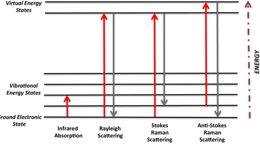
Raman spectroscopy is a scattering technique which differs substantially from other spectroscopic techniques. It is based on the non-polar scattering of occurrence radiation through interaction between laser light with a sample. The interaction will yield the molecular vibrations when the sample is illuminated by a monochromatic laser beam. The scattered light which have different frequency is used to construct a Raman spectrum. If scattered radiation has a frequency is equal frequency of incident radiation it constitutes Rayleigh scattering. The small fraction of scattered radiation which has a frequency different from frequency of incident radiation it is Raman scattering. When the frequency of incident radiation is higher than frequency of scattered radiation, Stokes lines appear in Raman spectrum. But when the frequency of incident radiation is lower than frequency of scattered radiation, anti-Stokes lines appear in Raman spectrum (G. S. Bumbrah and R. M. Sharma, 2016). [31]. The

(27)

spectrum generated by a Raman instrument generally has sharper and better resolved peaks than NIR which can provide more chemical information of unknown samples. Nevertheless, Raman spectroscopy requires more technical expertise (Strother and Todd, 2009) [32].

Figure 2.1. An energy level diagram illustrating the transitions occurring during Rayleigh scattering and Stokes and anti-Stokes Raman scattering (M. Baker, 2016) [33].

Raman spectroscopy is used in many varied fields. It can be used in any application such as non-destructive, miscroscopic, and chemical analysis. It can be utilaized to rapidly characterize the chemical composition and stracture of a sample such as solid, liquid, gas, gel, sellury or powder. In solid composition the common application are metal, glass, and plastic identification.

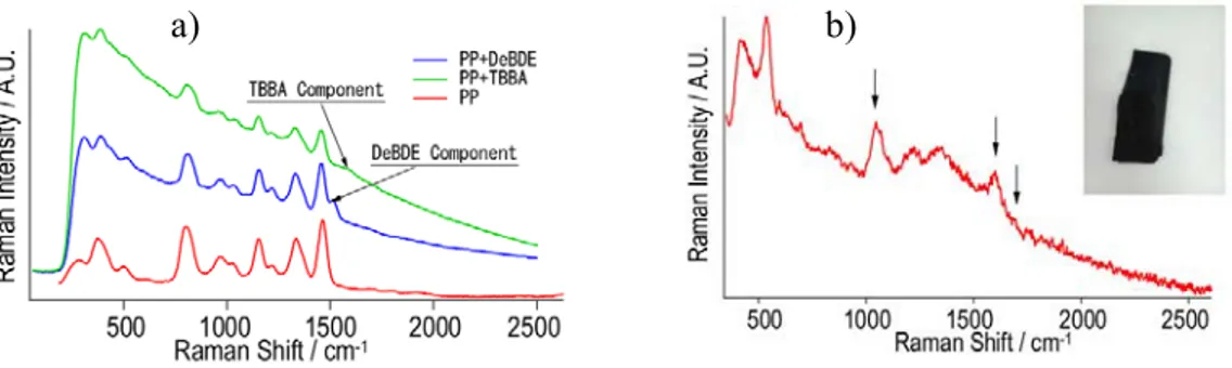
The application of Raman spectroscopy for plastic identification has condacted in several study. A. Tsuchida et at., (2013) [34] use portable Raman plastic

(28)

identifier which developed by Saimu Corporation to identify PET bottle, then PS, HIPS and AS which scanned as sample of similar plastics, DeBDE and TBBA mixed with PP are measured to show the detection of RoHS restricted substance. In Fig, 2.2 shows the Raman spectra of wet PET bottle and similar type of plastics, Fig. 2.3 displays the Raman spectra of bromine compounds on PP and black plastic.

Figure 2.2. a) Raman spectrum of wet PET bottle. b) Identification of similar type of plastics.

Figure 2.3. a) Identification of bromine compounds on PP. b) Identification of black plastic.

K. Carron and R. Cox, (2010) [35] in “Qualitative analysis and the answer box: A perspective on portable Raman spectroscopy” develop portable Raman spectroscopy to make the apparatus not esoteric, large, and expansive instrumentation.

a) b)

(29)

While maintaining the stability of laser for a stable specterum in x- and y-axis response and remain keep several factors such as laser temperature, injection current into the laser, and optical feedback, they have successed developing Raman spectroscopy which give information about characteristic of vibration molecular each plastic sample. In Fig. 2.4 illustrates the Raman spectra used to identify two plastics: polysulfone and polyethylene. The Raman spectroscopic signature equivalent to the odor is the 1148 cm-1 peak due to O=S=O symmetric sulfone stretching. This demonstrates how a Raman spectrum, just like the sniff test, provides answers to correctly identify a material. Consider the four styrenic plastics: polystyrene (PS), styrene butadiene (SB), styrene acrylonitrile (SAN), and acrylonitrile butadiene styrene (ABS). The Raman spectra of these four materials are shown in Fig. 2.5. All four materials exhibit similar Raman signatures due to a common styrenic functional group shared among the polymers. Though less intense than the styrenic regions, the highlighted regions at 715-825 cm-1 (red) and 1625-1700 cm-1 (blue) illustrate the differences among the materials. For example, the single peak observed in the blue region for ABS and SB is caused by thebutadiene carbon-carbon double bond.

Although the Raman spectroscopy easy and fast to give information about characteristic of plastic samples in form a spectra but still require computation techniques with algorithm combination that classification proses will running fast in idustrial scale.

(30)

Figure 2.4. Raman spectra of polysulfide (red) and polyethylene (green).

Figure 2.5. Raman spectra of styrene polymers: acrylonitrile butadiene styrene (ABS), styrene-butadiene (SB), polystyrene (PS), and styrene acrylonitrile (SAN).

Wavenumbers

(31)

2.3 Machine learning techniques

Automated learning often calls as Machine Learning (ML). It is a series process of mathematical analysis by computational complexity (algorithm) to learn input data which representing an experience and convert them to become an expertise or knowledge as an output (S. Shalev-Shwartz and S. Ben-David, 2014) [36].

Figure 2.6. The illustration of Machine Learning understanding.

In general, it can be described by the statistical learning framework as follows: a) The learner’s input which are consist of domain set, label set, and training data. The domain set is an arbitrary set with symbol 𝒳 which is the set of objects that may wish to label. The label set is the object that will restrict to be two-elements set,

normally {0,1} or {-1, +1} with symbol 𝒴. The training data: S = ((x1, y1) … (xm,

ym)) is a finite sequence of pairs of 𝒳 ⨉ 𝒴 that is a sequence of labeled domain

points.

b) The learner’s output is requested to output a prediction rule, h : 𝒳 → 𝒴. The function

is called a predictor, a hypothesis, or a classifier. The predictor and classifier can be used to predict or classify the label of new domain points.

input output

Dataset Model

computational

(32)

c) The training data are generated by some probability distribution with assume that

there is some correct labeling function, f: 𝒳 → 𝒴, and that yi = f(xi) for all i where

the labeling function is unknown to the learner. In summary, each pair in the training

data S is generated by first sampling a point xi according to 𝒟 a distribution over

some set and labeling it by f.

The importance of data preparation in machine learning is crucial factor to reduce error analysis in learning process. Hence, statistical properties as a technique which set up a modeling from probability distribution required to give valid training set. While, the right choice of learning algorithm will be an optimization technique which is used to seek the best parameters of the chosen model.

2.3.1. Principal Component Analysis

Principal component analysis (PCA) is probably the most popular multivariate statistical technique and it is used by almost all scientific disciplines (H. Abdi and L. J. Williams, 2010) [37]. According I. Jolliffe, (2011) [38] PCA is frequently possible to reduce the number of variables considerably while still retaining much of the information in the original data set. Therefore, it is probably the best known and most widely used dimension reducing technique. For instance, when the dataset has n measurements on a vector x of p random variables, and wish to reduce the dimension from p to q, where q is typically much smaller than p. PCA does this by finding linear combinations, 𝑎 𝑥, 𝑎 𝑥,…, 𝑎 𝑥, called principal components, that successively have maximum variance for the data, subject to being uncorrelated with previous 𝑎 𝑥𝑠. To

(33)

find solving the maximization problem can use the vector 𝑎 , 𝑎 , … , 𝑎 which are the eigenvectors of the covariance matrix S of the data, corresponding to the q largest eigenvalues. The eigenvalues give the variances of their respective principal components, and the ratio of the sum of the first q eigenvalues to the sum of the variances of all p original variables represents the proportion of the total variance in the original dataset accounted for by the first q principal components.

R. Bro and A. K. Smilde, (2014) [39] provide a description of how to understand, use, and interpret PCA which focuses in typical chemometric areas. They introduce the way of combining the original variables in a linier way which called a linear combination or weighted average. In Fig. 2.7. shows the concept of a unit vector. An important interpretation of PCA can be as a modelling activity.

𝑿 𝒕𝒑𝑻 _{𝑬 𝑿} _𝑬 _(2.1)

where X = a matrix, t = linear combination, p = the vector of regression coefficient, and E = matrix of residuals.

(34)

If the percentage of explained variation of equation 2.1 is too small, then the t, p combination is not sufficiently good summarizer of the data that suggests an extension the equation following:

𝑿 𝑻𝑷𝑻 _𝑬 _𝒕

𝟏𝒑𝟏𝑻 ⋯ 𝒕𝑹𝒑𝑹𝑻 𝑿 𝑬 (2.2)

where T = [𝑡 , … , 𝑡 ] (I x R) and P = [𝑝 , … , 𝑝 ] (J x R) are now matrices containing, respectively, R score vectors and R loading vectors.

Figure 2.8 The structure of PCA model.

2.3.2. Support Vector Machine

Support Vector Machine (SVM) is a useful algorithmic of machine learning which can solve regression, clustering dan classification problem. It is not only for learning linear predictors but also nonlinear predictors in high dimensional feature space which will increase both sample complexity and computational complexity challenges.

(35)

The principal of SVM algorithm is to separate two classes or more of sample complexity challenge by searching maximum margin separators between support vector from each class with optimum hyperplane. The optimum hyperplane is a linear or nonlinear line which separate the classes and it is the core of SVM. In Fig. 2.9 displays the illustration the SVM classification.

Figure 2.9. The illustration of SVM, a) plot of dataset red and blue classes, b) the optimum hyperplane with maximum margin between support vector. In the theory of SVM (M. O. Stitson, et al, 1996) [40] explaints that determine

a separating hyperplane is given 𝑥 , 𝑦 , … , 𝑥 , 𝑦 , 𝑥 ∈ 𝑅 , 𝑦 ∈ 1, 1 by the

training data with optimum hyperplane is 𝑤. 𝑥 𝑏 0 . To find it, requiere

calculating hyperplane in each class side as a boundary with equation is following:

𝑤. 𝑥 𝑏 1, 𝑖𝑓 𝑦 1 (2.3)

𝑤. 𝑥 𝑏 1, 𝑖𝑓 𝑦 1 (2.4)

where 𝑤 is a margin from the boundary of support vector to optimum hyperplane and 𝑏 is a constant factor or bias.

red class

blue class

support vector

(36)

The calculation optimum hyperplane is based on maximizes the minimum distance between hyperplane (boundary) of the training data by equation following:

𝜌 𝑤, 𝑏 _{𝑥 |𝑦}𝑚𝑖𝑛 ₁ . _{| |} _{𝑥 |𝑦}𝑚𝑎𝑥 ₁ . _{| |} (2.5)

The sum of the distance from the nearest two points to separating hyperplane which must be maximized. From equation 2.5 and equation 2.3 can be described follows:

𝜌 𝑤, 𝑏 _{𝑥 |𝑦}𝑚𝑖𝑛 ₁_{| |} _{𝑥 |𝑦}𝑚𝑎𝑥 ₁_{| |} (2.6)

⇔ 𝜌 𝑤, 𝑏 _{| |} _{| |} (2.7)

⇔ 𝜌 𝑤, 𝑏 _{| |} (2.8)

⇔ 𝜌 𝑤, 𝑏

√ . (2.9)

The optimum hyperplane therefore minimizes

Φ 𝑤 𝑤 . 𝑤

To solve this problem can be found by finding the saddle point of the Lagrange functional:

𝐿 𝑤, 𝑏, 𝛼 𝑤 . 𝑤 ∑ 𝛼 𝑥 . 𝑤 𝑏 𝑦 1 (2.10)

where 𝛼 are Lagrange multipliers. The Lagrange must be minimized with respect to

𝑤, 𝑏 and maximized with respect to 𝛼 0.

In the saddle point the solutions 𝑤 , 𝑏 , and 𝛼 should satisfy the following condition: , ,

0 (2.11)

(37)

, , ₀ _(2.13)

⇔ 𝑤 ∑ 𝛼 𝑥 𝑦 0 (2.14)

The result of optimum hyperplane in the following properties: 1. Constraint on the coefficients 𝛼 from equation 2.12:

∑ 𝛼 𝑦 0, 𝛼 0, 𝑖 1, … , 𝑙 (2.15)

2. The vector 𝑤 is a linear combination of the vectors in the training set (from

equation 2.14):

𝑤 ∑ 𝛼 𝑥 𝑦 , 𝛼 0, 𝑖 1, … , 𝑙 (2.16)

3. Only the so-called support vectors can have non-zero coefficient 𝛼 in the

expansion of 𝑤 :

𝑤 _{𝑠𝑢𝑝𝑝𝑜𝑟𝑡 𝑣𝑒𝑐𝑡𝑜𝑟𝑠 𝛼 𝑦 𝑥 , 𝛼}∑ 0 (2.17)

The Kuhn-Tucker Theorem state that the necessary and enough condition for the optimal hyperplane are that the separating hyperplane satisfies the conditions:

𝛼 𝑥 . 𝑤 𝑏 𝑦 1 0, 𝑖 1, … , 𝑙 (2.18)

Substituting these results into the Lagrange, the following functional is obtained:

𝑊 𝛼 𝑤 . 𝑤 ∑ 𝛼 𝑥 . 𝑤 𝑏 𝑦 1 (2.19)

𝑤 . 𝑤 ∑ 𝛼 𝑦 𝑥 . 𝑤 𝑏 ∑ 𝛼 𝑦 ∑ 𝛼 (2.20)

𝑤 . 𝑤 𝑤 . 𝑤 0 ∑ 𝛼 (2.21)

(38)

The functional must be maximized in the non-negative quadrant,

𝛼 0, 𝑖 1, … , 𝑙 (2.23)

under the constraint

∑ 𝛼 𝑦 0 (2.24)

Once the solution to the problem has been found in form of a vector 𝛼 𝛼 , … , 𝛼 ,

an indicator function can be constructed:

𝑓 𝑥 𝑠𝑖𝑔𝑛 _{𝑠𝑢𝑝𝑝𝑜𝑟𝑡 𝑣𝑒𝑐𝑡𝑜𝑟𝑠 𝑦 𝛼 𝑥 . 𝑥}∑ 𝑏 (2.25)

where 𝑥 are the support vectors, 𝛼 are the Lagrange multipliers and the 𝑏 is the threshold

𝑏 𝑤 . 𝑥∗ ₁ _{𝑤 . 𝑥}∗ ₁ _(2.26)

where 𝑥∗ _{1 is any support vector belonging to the first class and 𝑥}∗ _{1 is any}

support vector belonging the second class.

Modified for non-separable data 𝛼 must be bounded:

0 𝛼 𝐶 (2.27)

where C is a constant chosen a priori. 2.3.3. Artificial Neural Network

Artificial neural network (ANN) is a classification machine learning technique which inspired from the human brain structure and biological brain neural networks. The aim is to simulate human intelligence, reasoning and memory to solve forecasting, pattern recognition and classification problems. The idea behind neural networks is that

(39)

many neurons can be joined by communication links to carry out complex computations. The structure of a neural network as a graph whose nodes are the neurons and each (directed) edge in the graph links the output of some neuron to the input another neuron (S. Shalev-Shwartz and S. Ben-David, 2014) [36].

Figure 2.10. The illustration of ANN concept, a) the biological brain neural netwoks struture, b) the simulate of biological brain to ANN algorithm.

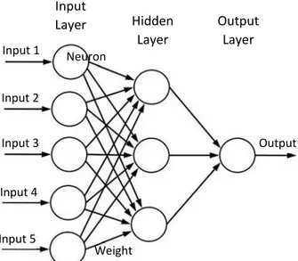
According G. M. Khan (2018) [41] the arcitecture of an artificial neural networks consist of an input layer of neurons (or nodes, unit), one or two (or even three) hidden layers of neurons, and final layer of output neurons. Fig. 2.11 shows the architecture of ANN with lines neruron connection which is associated by numeric

number called weight. The output ℎ of neuron 𝑖 in the hidden layer is folowing:

ℎ 𝜎 ∑ 𝑉 𝑥 𝑇 (2.28)

where 𝜎 is called activation function, 𝑁 the number of input neurons, 𝑉 the weight,

𝑥 inputs to the input neurons, and 𝑇 the threshold terms of the hidden neurons. The

purpose of activation function is to bound the value of the neuron that the neural network is not paralyzed by divergent neurons.

(40)

Figure 2.11 Architecture of artificial neural networks

The activation function is one of principal factors which will affect the performance of the networks. It used to transform the activation level of a neuron (node) into an output signal. Many types of activation funtion, but basically it can be divided into two types, linear activation function and non-linear activation function ( J. Feng and S. Lu, 2019) [42], (B. Karlik and A. V. Olgac, 2011) [43]. The common activation function is as following:

1. Linear activation function

Linear activation function has the equation similar to as of a stright line which is proportional to input and it is given by,

𝑓 𝑥 𝑘𝑥 (2.29) Input Layer Hidden Layer Output Layer Input 1 Input 2 Input 3 Input 4 Input 5 Output Neuron Weight

(41)

where 𝑥 is the input of the activation function 𝑓 on the 𝑖 th chanel, and 𝑘 is a fixed constant, 𝑓 𝑥 is the corresponding output of the input.

2. Uni-polar Sigmoid Function

Uni-polar Sigmoid Function is a non-linear actifation function that especially advantageous to use in neural networks trained by back-propagation algorithm. It is easy to distinguish and can interestingly minimize the computation capacity for training. The equation is given as follows:

𝑓 𝑥 (2.30)

3. Bi-polar Sigmoid Function

Activation function Bi-polar Sigmoid similar with Uni-polar sigmoid, but it goes well for applications that produce output values in the range of [1.-1]. The equation is as following:

𝑓 𝑥 (2.31)

4. Tanh Function

Tanh function also known as Tangent Hyporbolic Funtion, it can obtained from Sigmoid Function, it is given by,

tanh 𝑥 1 2𝑠𝑖𝑔𝑚𝑜𝑖𝑑 2𝑥 1,

(42)

5. ReLu

ReLu has become very populer in the last few years which is usually implemented in hidden layers of ANNs, especially in almost all the Conventional Neural Networks (CNN) or Deep Learning (DP), it is given by,

𝑓 𝑥 max 0, 𝑥 𝑥 , 𝑥_{0, 𝑥} _{0 , 𝑓 𝑥}0 1, 𝑥_{0, 𝑥} 0₀ (2.33)

2.4 Machine learning technique in industrial field

Nowadays, in many countries have announced a new round of development plans in industrial manufacturing to achieve efficiency processing for the future by technology. It is means how to increase energy efficiency, reduction of CO2 emissions, renewable, revitalization plan for manufacturing, and even propose the concept industry 4.0. All the action intends to improve whole aspect of the industrial process, such as sustainability design, system integrator, advanced process/quality control, decision supports, etc. A large amount of data has been achieved in the process industry due to the wide use of distributed production and control system.

According Z. Ge, et al, (2017) [44] that data mining and analytics by machine learning technique will increase the handling of complex process, data-driven process modeling, monitoring, prediction and controlling. Furthemore, they itemize that there are two types method of machine learning technique which applied in the process industry i.e. unsupervised learning methods and supervised learning methods. Fig 2.12 shows the percentages of unsupervised learning techniques in different aspects, while

(43)

in Fig 2.13 displays the persentages of supervised learning techniques which implemented in different aspects.

Figure 2.12. The percentages of application statuses of unsupervised learning techniques in dimensionality reduction, outlier detection, process monitoring, and data visualization [44].

In a study concerning Rethinking Human-Machine Learning in Industry 4.0, F. Ansari, et al, (2018) [45] explain that from a computer perspective, artificial model and computational algorithm resemble the ability of human learning and produce human skill. The model building as a core of the process is automated using methods machine learning to identify new learning patterns in highly digitalize industrial work scenarios for factory industry 4.0.

Dimensionality reduction Outlier detection

Data visualization Process monitoring

(44)

Figure 2.13. The percentages of supervised learning techniques which is implementing in industry to handle process monitoring, fault classification, soft sensor, and quality prediction [44].

Process monitoring Fault classification

(45)

Chapter 3 Experimental of Plastic Identification

In this study, we identify three types of plastic i.e. Polypropylene (PP), Polystyrene (PS), and Acrylonitrile Butadiene Styrene (ABS). The number of samples are 101 which consist of 50 PP, 32 PS, and 19 ABS from electric appliance used plastics. The flow of experimental illustrates in Fig. 3.1 which begin with data preparation that are peak extraction, data normalization, and adding noise. Original dataset used as data training and testing for SVM techniques, data training for PCA-SVM and ANNs techniques, while dataset which added noise used as data testing for PCA-SVM and ANNs techniques.

3.1 Correction of Raman spectra of waste plastics

The type of them has detected by molecular chains produced frequencies of different torsion vibration using Raman spectroscopy that higher laser diode (785 nm, 1W) and high throughput optical system, highly sensitive back-illuminated FFT-CCD (1024 pixels), and onboard digital signal processing system with identification speed within 6 ms to address the considered noise level. Each correct plastic resin type was verified by using the Fourier Transform Infrared Spectroscopy (FT-IR) measurement. 3.2 Software

To support the experiment running well, we use computer application and language programming to process and analyze of data which has collected. Microsoft excel in format CSV used to store the data from Raman measurement and use as manual

(46)

calculation to evaluate values from R dan Python. SVM and PCA analysis use R with library e1071, ggplot2, and ggfortify. Python programming language used to peak extraction, baseline reduction, make and add noise into spectra and calculate margin between support vector.

3.3 Peak extraction

The Raman spectra from measurement process consists of many peaks in

range 0 – 3600 cm-1_{which is caused by molecule vibration when the material receive}

light energy that indicate the chemical characteristic of the material. To obtain dataset for analysis was done peak extraction by several steps: essential peaks selection, baseline reduction, and peak area calculation.

3.3.1 Essential peaks selection

To make the analysis may be running fast, then selected four essential peaks which can be explicitly distinguish each plastic type. Fig 3.2 shows the peaks selection

of the Raman spectra, where peak 1 of C-H bending at 820 cm-1_{/ 165}th_{pixel, peak 2}

of benzene ring berating at 1000 cm-1_{/ 208}th_{pixel, peak 3 of C=C stretch at 1600 cm}-1

/ 373rd_{pixel, and peak 4 of C=N stretch at 2240 cm}-1_{/ 580}th_pixel.

The pixel position of peak 1 – 4 is a start point to calculate peak value in each peak for the dataset. For each start point is sought minimum value of the left side as 𝑥 pixel and minimum value of the right side as 𝑦 pixel. The 𝑥, 𝑦 pixel is a boundary of peak area which will use to baseline reduction.

(47)

Figure 3.1. The experimental scheme of plastic identification.

Figure 3.2. Essential peaks selection in ABS, PP, and PS spectra. Data normalization Dataset Shredded waste plastics Sample initialization 61 PP, 33 PS, 21 ABS Raman measurement Raman spectra Essential peaks extraction Adding noise 0.75, 1.5, 2.5, 3.75, 7.5, 15‐times (dataset) 70 % d ata tr ainin g, 30% data testin g dat a t raini n g PCA‐SVM dat a testin g SVM ANNs Plastic classification A B C A B C

(48)

3.3.2 Baseline reduction

To keep the performance is remain running fast, baseline reduction uses simple technique by subtraction entire intensity values in peak area between 𝑥 and 𝑦 pixel with background value which is obtained from an equation as follows:

𝑏𝑔 (3.1)

where 𝑥 is average of value from 𝑥 pixel until 10 pixels before 𝑥, while 𝑦 is average of value from pixel until 10 pixels after 𝑦, and 𝑏𝑔 is background value. In subtraction process minus value will be ignored. Fig 3.3 shows the illustration of baseline reduction.

Figure 3.3. Illustration of baseline reduction. 3.3.3 Peak area calculation

The last step of peak extraction is calculation of peak area after baseline reduction. It is done using trapezoidal rule [46] that given by,

𝑇 ∆ 𝑓 𝑥 2𝑓 𝑥 ⋯ 2𝑓 𝑥 𝑓 𝑥 (3.2)

(49)

where 𝑇 is the value of data after peak extraction, 𝑓 𝑥 is intensity value of 𝑖-pixel, while 𝑎 is the beginning of pixel, 𝑏 is the end of pixel, 𝑛 is amount of pixel in peak area. In which ∆𝑥 will always equal 1, because the minus value ignored when baseline reduction was processing.

The peak extraction yields four-dimension dataset i.e. P1, P2, P3, and P4 which came from extraction peak 1, peak 2, peak 3, and peak 4.

3.4 Data normalization

Normalization is a step that often applied to prepare dataset for machine learning. The aim of it is to change the intensity value of numeric columns in the dataset to a common scale without distorting differences in the range of values. In our experimental, due to the data is identical which came from Raman spectra, so we prepare the dataset using normalization technique by equation as follows:

𝑑𝑠 _∑ (3.4)

where 𝑑𝑠 is data normalize of 𝑖-column, 𝑥 is data that will normalize of 𝑖-column,

and ∑ 𝑥 is amount data of all columns.

Now, we have dataset that called original dataset which will use as data training for all machine learning techniques in our study and as data testing for SVM technique and dataset that has added noise as data testing. The original dataset can be seen in appendix pages.

(50)

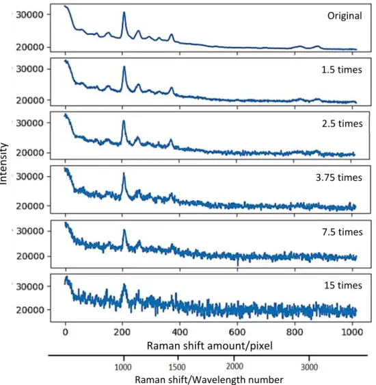
The goal of adding noise is to examine the robustness of classification model that can applied on industrial field, because in industry scale the processing often prone to disturb by external noise such as the material mixing or contaminate with others material, and internal noise may come from the frequency that produced by others device.

To prepare dataset for data testing to PCA-SVM and ANNs techniques, we were adding noise on the Raman spectra with several steps i.e. trigger random values by Gaussian distribution that called noise, adjust intensity magnification of noise signal, and add the noise signal to the original dataset. The equation is following:

𝑝 𝑥 _√ 𝑒𝑥𝑝 (3.5)

𝑠𝑝𝑛 𝑖𝑛𝑡 ∗ 𝑝 𝑥 𝑠𝑝 (3.6)

where 𝑝 𝑥 is noise signal with 𝜇 = 0 and 𝜎 = 1, 𝑥 is pixel, 𝑠𝑝𝑛 spectra have added noise, 𝑖𝑛𝑡 is magnification value, and 𝑠𝑝 is original Raman spectra. In Fig. 3.4. shows the signal that triggered by Gaussian distribution.

(51)

The spectra which has added noise will treat similar steps such as original dataset to obtain new dataset that uses as data testing for PCA-SVM and ANNs. In Fig. 3.5. display the spectra which has been adding noise

In the wake of the dataset was available for analysis using machine learning to obtain new method for plastic identification which can be implemented in industrial field. The dataset which has added noise can be seen in appendix pages. Whole process

Figure 3.5. The Raman spectra of Polystyrene (PS), original and after adding noise.

Intensity Original 1.5 times 2.5 times 3.75 times 7.5 times 15 times Raman shift/Wavelength number Raman shift amount/pixel

(52)

of data preparation is established by using application which constructed using Python language programming with utilize few mathematic and statistics libraries such as NumPy, Pandas, Math, and Matplotlib, and Python framework PyQt 5.

(53)

Chapter 4 Plastic Identification using SVM Technique and

PCA-SVM Integration Techniques

In this section we will explain deeply about our approach using machine learning techniques in choosing peaks of Raman spectra without expertise spectroscopic knowledge and how the machine learning work to retrieve important information from Raman spectra to classify the type plastics. The approaches are useful for industrial field, especially in recycling industry. The explanation we will clear up into two section which is main of our study.

From the dataset which has explained the preparation in previous chapter, it will be used as analysis foundation using machine learning techniques to gain effectiveness of the techniques for plastic identification especially in industrial field. The exposure in this chapter is divided into two section. First, performance of SVM algorithm to plastic identification using combination of four essential peaks that is discovered prime combination of peaks pair to distinguish the type of plastic. Second, achievement of PCA-SVM integration which uses whole of essential peaks to generate classification robustness model by adding noise signal which represent real condition of industrial.

Entire of the analysis supported by using R programming which apply e1071, ggplot2, factorMineR, factoextra, and corrplot library for SVM and PCA analysis, while for ANNs analysis used Python language programming which adjust Keras library.

(54)

4.1. Quantitative Evaluation for the Peak Selection in the Raman Spectroscopy Classification of Plastics Based on the SVM

Raman spectroscopy has recently been used for material identification in industrial sites and for research work in laboratories. The measurement of Raman spectra provides rapid and accurate identification and is conducted by using contactless

optical alignment to scattering light. Furthermore, Raman apparatus has generally

become more compact and cheaper, owing to the development of semiconductor lasers and optical devices such as deposition filters. The Raman spectral peaks imply intrinsic molecular vibrational information, which could be obtained by applying infrared absorption spectroscopy. We have developed a practical plastic waste sorting system applicable at an industrial scale by adopting these features of Raman spectroscopy.

Raman spectroscopic identification offers several advantages for mechanical recycling compared to the near infrared absorption (NIR) technique, which is widely used for plastic sorting purposes in industry. The purity of resin sorted out using the proposed approach is close to 98%, owing to the sharp and distinct Raman peaks and minor noise due to water. In turn, the NIR spectra are characterized with broad and indistinct peaks and large background noise due to water in the wide spectral range. The suggested Raman identification apparatus operates with a fast measurement time of 3 ms for each spectrum of plastic waste from used home appliances: polypropylene (PP), polystyrene (PS), and acrylonitrile- butadiene-styrene copolymer (ABS). In this method, 25 identifiers in parallel operations can process shredded plastic flakes (5–30 mm) on the conveyor belt with a throughput speed of 400 Kg/h.

(55)

The spectra obtained during a very short measurement time include a large amount of white noise, and the existence of spectroscopic peaks may become ambiguous. Several multivariate analysis approaches (such as a neural network technique) have been employed to achieve accurate identification. However, the spectroscopic data must be analyzed in real-time for industrial applications. During the classification of a massive amount of waste plastic, a simpler and faster identification method is required, such as a method based on straightforward comparison of peak intensities without multivariate analysis, rather than a method that requires complex matrix calculations and considerable computing resources.

This study demonstrates a way of applying the machine learning method based on the support vector machine (SVM) to perform quantitative evaluation of the spectral peaks to select the decisive and representative peaks in the Raman spectra without the need for expert spectroscopic knowledge. Effective categorization of three types of plastic (PP, PS, and ABS) was achieved by the intensities of only two selected peaks. Common approaches based on the Raman or IR spectrum analysis imply that we search for the representative peaks corresponding to the characteristic vibration modes in a molecule using the theoretical and/or empirical spectroscopic information. In some cases, this process is subject to the trial-and-error procedure. The multivariate analysis of plural peaks in the spectra also becomes a versatile approach used for the identification with the rapid development of computation technologies. However, computationally expensive methods requiring complicated calculations do not allow rapid identification with a processing speed in the range of several milliseconds.

(56)

With using dataset that consist of P1, P2, P3, and P4 which obtained from peak 1, peak 2, peak 3, and peak 4 respectively that arranged into six combination of peak pairs i.e. P1-P2, P1-P3, P1-P4, P2-P3, P2-P4, and P3-P4. Each of peak pairs analyzed using SVM technique to find superlative plastic type separation. SVM will use data training to find out optimal hyperplane in vector space which will distinguish every classes of plastic (PP, PS, and ABS) from each peak pair. In training process of SVM will determine optimum hyperplane which separate the class, maximum margin between support vector, amount of support vector in each class, and the number of data that suitable with class area or mis area. While, data testing used as indication of accuracy of new data toward SVM classification model that establish along training process.

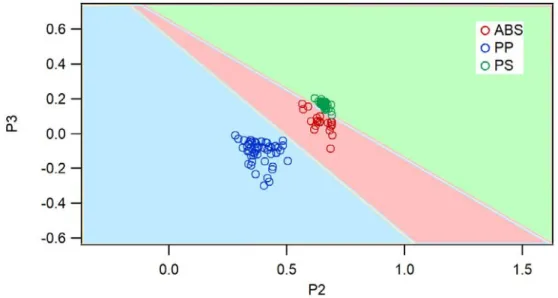
In this study we use multiclass linear SVM, in other words the shape of hyperplane which discriminate the classes is straight line, even though the real plot representation not exactly. Due to there are three classes discrimination, we use three color to identify each class area. Blue area is PP class, green area is PS class, and red area is ABS class. The color of node similar with color area, yet it is just darker.

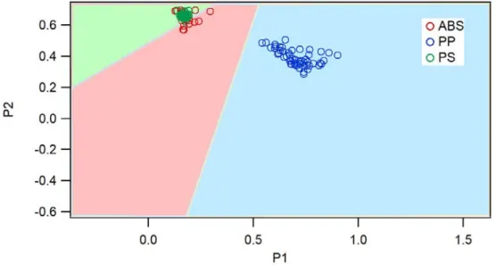
In Fig. 4.1 shows the SVM plot classification of peaks pair P1 and P2. The margin between support vector that clear identify is only midst PP and ABS i.e. 0.356, while others margin could not be identified clearly which caused coordinate of PS and ABS relatively similar. The total number of support vector that used to create the optimum hyperplane is 19 support vectors which consist of PP = 1, PS = 8, and ABS = 10. The accuracy of SVM classification model is 0.88 or around 88%.