A learning algorithm for monotone $k$-term DNF

84

A learning algorithm for monotone k-term DNF

Takeshi

OHGURO

Akira

MARUOKA

(

大黒毅

)

(

丸岡章

)

Department of

Information Engineering,

Faculty of

Engineering,

Tohoku

University

Abstract

Recently, Valiant introduced a computational model oflearning, and gave a precice

definition of learnabihty. Since then, much effort has been devoted to characterize learnable classes of concepts onthis model. In this paper, we give, based on the

uni-form distribution model, a polynomial time algorithm that learns k-term MDNF, the class of monotone disjunctive normal formulae with at most $k$ terms. This algorithm

uses only positive examples and output hypothesis with one-sided-error. This result should be contrasted with the fact that the same class is not learnable in the dis-tribution free setting. Based on the uniform distribution model, learning algorithms

for k-term MDNF were given in [GM,KMP]. But these algorithms use both positive and negative examples. Consequently error of these algorithms is two-sided.

Fur-thermore, the algonithm proposed in this paper is easily modifiedto learn the same

class in thepresence oferrors in the examples.

1

Introduction

Recently, Valiant introduced a computational model of learning, and gave a precice def-inition of learnability based on the model [V84]. A class of Boolean formulae is said to be learnable if there exists a polynomial time algorithm to learn any formula in the class: With access to oracles that give some partial information about an unknown target for-mula in the class, the learning algorithm outputs a Boolean formula that is, with high

likelihood, a reasonably accurate approximation to the target. Since Valiant has proposed this learnability model, much effort has been devoted to characterize learnable classes.

In particular, several algorithmsto learnclasses ofBoolean formulae from examples have been studied (see $[KLPV87a,H]$ for example). Among these, the problem oflearning the

class of disjunctive normal forms (DNF) seems to be important. But whether DNF is learnable from examples is open in the distribution free model. The same problemremains open even if we restrict ourselves to the distribution specific model, where positive or

negative examples of$f$ are generated according to the uniform probability distributions.

数理解析研究所講究録 第 731 巻 1990 年 84-96

85

In this paper we give, based on the uniform distribution model, a polynolnial time

algorithm

to learn k-term MDNF, the class of monotone disjunctive normal formulae with

at most $k$ terms, from positive examples. This result should

be

contrasted with the fact

that the same class is not learnable in the distribution free setting [PV].

Based on the uniform distribution model, learning algorithms for k-term MDNF have

been proposed in literature. In [GM] a learning algorithm for k-term MDNF is given. A

more

natural algorithm was proposed in [KMP]. But the crucial part of the algorithm,

hence the probabihty analysis to show its correctness, was not given in the paper.

The idea of the learning algorithm, givenin this paper, for k-term MDNF is based on one of the learning algorithm givenin [KMP], although one of the key ideas ofrestricting the domain where a target function is identified was not mentioned explicitly in [KMP]. Using the idea of restrictions carefully, we can construct the learning algorithm that is assumed to use only positive examples, whereas the algorithms given previously in literature

were

assumed to use both positive and negative examples. Consequently, the type of error for the algorithm of this paper is one-sided, while that for the previous algorithms is two-sided.

We give the whole algorithm explicitly together with the proof of its correctness.

Furthermore, the algorithm proposed in this paper is easily modified to learn the same class in the presence of errors in the examples.

2

Preliminaries

We first describe the Valiant’s model for learning that we shall use briefly. For more

complete discussion and justification of the model, see [PV], [V84] and $[KLPV87b]$.

Let $F_{n}$ be a set of formulae with variables $\{x_{1}, \ldots, x_{n}\}$, and let $F=\cup F_{n}$. Let $f$ be a

formula in $F_{n}$. For convenience, we regard $f$ in $F_{n}$ as the corresponding Boolean function

with domain $\{0,1\}^{n}$, and sometimes as the set of vectors such that $\{v|f(v)=1\}$. A vector $v\in\{0,1\}^{n}$ is called a positive example (resp. negative example) of $f$ iff $f(v)=1$ (resp.

$f(v)=0)$. $D_{f}^{+}$ (resp. $D_{f}^{-}$) is a probability distribution uniform over all positive (resp.

negative) examples of$f$. $D_{f}^{+}(D_{f}^{-})$ is simply written as $D^{+}(D^{-})$ when no confusion arises.

In this paper a learning algorithm is assumed to call an oracle $POS(f)$, which produces positive examples of$f$independently according to the probabilitydistribution $D_{f}^{+}$. $POS(f)$

is simply written as POS when no confusion arises. In more general setting, the learning algorithm is also allowed to call another type of oracles (e.g. $NEG(f)$, which produces

negative examples). We adopt the distribution specific model where the probability that examples are generated is taken to be uniform, whereas in the distribution free model the probability is taken to be arbitrary. But in fact, the condition that $D^{-}$ is uniform is not

necessary for the algorithm giveninthis paper: It works as well when $D^{-}$ is taken arbitrary.

Definition. Aclass of formulae $F$is called learnable if there exists an algorithm $L_{F}$, with

86

$\forall n,$ $\forall f\in F_{n},$ $\forall\delta,$ $\forall\epsilon$,

i) $L_{F}$ runs in time polynomial in _$n,$ $\frac{1}{\epsilon}$ and $\frac{1}{\delta}$

ii) $L_{F}$ outputs a formula $g$ in $F_{n}$ with probability at least 1 $-\delta$, that satisfies

$\Sigma_{g(v)=0}D^{+}(v)<\epsilon$ and $\Sigma_{g(v)=1}D^{-}(v)=0$.

$f$ is called a target

formula

and $g$ is called a hypothesis. $\epsilon$ is called a accuracy parameter

and $\delta$ is called a

confidence

parameter. According to the definition we simply say $F$ is

learnable instead of saying $F$ is polinomial time learnable from positive examples under uniform distributions with one-sided-error.

A conjunction of litelals is called a monomial (or a term). For constant $k$, let k-term

MDNF denote the class of monotone disjunctive normal forms with up to $k$ terms. Let

$Var(t)$ denote the set of variables that appearin monotone term $t$. Let Term$(f)$ denote the

set ofterms of a formula $f$. Let $v_{i}$ denotes the ith component of $v$. Likewise, let $v_{A}$ denote

the $i_{1},$$i_{2},$

$\ldots$, and $i_{j}$th components of$v$, where $A$ is a subset $\{x_{t_{1}}, \ldots, x_{i_{j}}\}$ of $\{x_{1}, \ldots, x_{n}\}$.

$v_{A}=0$ means that $v_{i_{1}}=\cdots=v_{i_{j}}=0$

.

Next we describe some results useful in probabilistic analysis in this and subsequent sections. Let LE$(p, m, r)$ denote the probability of at most $r$ successes in $m$ independent trials with probability of success at least $p$, and $GE(p, m, r)$ denote the probability of at

least $r$ successes with probability ofsuccess at most $p$.

Let $b$ be such that _{$0\leq b\leq 1$} in the following facts.

Fact 2.1 $[KLPV87b]$ LE$(p, m, (1-b)pm)\leq e^{-b^{2}mp/2}$.

Fact 2.2 $[KLPV87b]$ $GE(p, m, (1+b)pm)\leq e^{-b^{2}mp/3}$.

Proposition 2.3 [V84] LE$(p, m, r)\leq 6$ for $m \geq\frac{2}{p}(r+\ln\frac{1}{\delta})$.

Procedure EXAMPLES given in Figure 1 produces a sequence of $m$ positive examples

which satisfy the condition $C(v)$. The condition ‘TRUE’ always holds: It means that there

is no spacific condition. $|S|$ denotes the length of the sequence $S$. As in the definition of

learnability,

6

is called

_confidence

parameter of EXAMPLES.

Proposition 2.4 Let

$0<6<1$

. If $Pr[C(v)]\geq p_{c}$, then EXAMPLES produces a

sequence $S$ of _$m$ positive examples which satisfy the condition _$C(v)$, with probability at

least

1–6.

If the condition $C(v)$ is TRUE then the probability is 1.

Proof. Immediate from Proposition 2.3. $\square$

Note that all positive examples in $S$ are independently taken from uniform distribution over the positive examples satisfying the condition $C(v)$.

Procedure FREQ given in Figure 2 can be used toestimate the probability of event $E(v)$

87

procedure

EXAMPLES(m, $C(v),$ $p_{c},$ $6$)

begin

let $S$ be a empty sequence ;

if $C(v)=TRUE$ then $m’$ _$:=m$

else $m’$ $:= \frac{2}{p_{c}}(m+\ln\frac{1}{\delta})$ ;

for $c:=1$ to $m’$ do

begin

$v:=POS$ ;

if $C(v)$ holds then add $v$ to $S$ ;

end return $S$ ;

end

Figure 1: Procedure EXAMPLES

procedure FREQ$(S, p-\alpha, p, E(v))$

begin

$c$ $:=0$ ;

foreach $v$ in $S$ do if $E(v)$ holds then $c:=c+1$ ;

if $c\geq|S|(p-\alpha/2)$ then return “high” else return (low’ _;

end

Figure 2: Procedure FREQ

Lemma 2.5 Let $\alpha,$ $p$ be such that $0<p \leq 1,0<\alpha\leq\frac{2}{3}p$ and $0<\delta<1$. Let $S$

be a sequence of $m$ vectors which are drawn independently according to some distribution

(probabilityis measured by this distribution). Let $m$ satisfies thefollowing condition (2-1).

$m \geq\max\{\alpha 8\lrcorner_{2}\geq\ln\frac{1}{\delta},$ $\frac{12(p-\alpha)}{\alpha^{2}}\ln\frac{1}{\delta}\}$ (2-1)

Then, if $Pr[E(v)]\leq p-\alpha$ then FREQ returns “high” with probability at most 6, and if

$Pr[E(v)]\geq p$ then FREQ returns (low’ _{with probability at most}

_6.

$b= \alpha/2(p-\alpha),itfollowsthatGE(p-\alpha,m,(p-\alpha/2)m\exp-\{\frac{d_{\alpha}u}{2(p-\alpha)}\}^{2}(p-\alpha)\frac{.12(p-\alpha)2with}{\alpha^{2}}Proof.AssumethatPr[E(v)]\leq p-\alpha.Takingm=\frac{12(p-\alpha)}{)\leq^{2}\alpha}\ln\frac{1}{f}ansingFact2$

. .$\ln\frac{1}{\delta}/3]=\delta$. Therefore, the probability that $E(v)$ holds at least $(p-\alpha/2)m$ times among

$m$ independent trials is at most

6.

Thus FREQ returns $\zeta high$’ with probability at most

6.

For the second part of the Lemma, assume that $Pr[E(v)]\geq p$. Taking $m= \not\in 8\alpha\ln\frac{1}{}$ and

using Fact 2.1 with $b=\alpha/2p$ as above, it can be seen that the probability that $E(v)$ holds

at most $(p-\alpha/2)m$ times among $m$ independent trials is at most $\delta$. Therefore FREQ

returns (low’ _{with probability at most}

_6.

Since theupper bounds givenin Fact 2.1 and Fact 2.2 are monotonedecreacing functinos

88

$\delta$ is called

confidence

parameter of FREQ. In later sections, Lemma 2.5 will be used

to estimate the probabihty of $E(v)$ from the value procedure FREQ returns: With high

confidence the fact that FREQ returns “low” implies that $Pr[E(v)]<p$, and

the

fact

that FREQ returns (high’ implies that $Pr[E(v)]>p\neg\alpha$. This is because both of the

probability of occurrence of (low’ _and $Pr[E(v)]\geq p$, and that ofoccurrence of “high” and $Pr[E(v)]\leq p-\alpha$ are at most 6, which will be taken sufficiently snall in the following

argument. To simplify the argument in section 4, we say that “low” implies $Pr[E(v)]<p$

and that “high” implies $Pr[E(v)]>p-\alpha$. We only take care of the probability 6 at the end of the argument.

In some cases, we need to estimate the conditional probability of event $E(v)$ under some

condition$C(v)$. This is done by combining procedure EXAMPLES and FREQ. In this case,

EXAMPLES does not always succeed in producing the desired sequence $S$, but succeed in

with high probability. In section 4, we omit the phrase “with high probability” and treat as if EXAMPLES always produces the desired sequence for simplicity. We only take care of the probability of failure at the end of the argument, as is the case for FREQ.

3

Learning

algorithm for k-term MDNF

Before proceeding to describe the learning algorithm $L$ for k-term MDNF in detail, we give

an outline of the $al$gorithm together with an idea behind it.

Let $f=t_{1}\vee t_{2}\vee\cdots\vee t_{k}$ be a target in k-term MDNF. Without loss of generality, assume that none of the terms of $f$ is redundant in the sense of being implied by the sum of the

others. Fact 3.1 below is the basis of the algorithm: In order to find out a term$t$ which is

not found yet, the algorithm attempts to determine such a set $A$ as in the fact.

Fact 3.1 Let$f$ be anon-redunduntformula in k-term MDNF. For any term$t$ in Term$(f)$,

there exists a set $A$ of variables such that $A\cap Var(t)=\emptyset,$ $A\cap Var(t’)\neq\emptyset$ for any term$t’$

in Term$(f)-\{t\}$, and $|A|\leq k-1$.

Suppose that algorithm $L$ succeeded in producing the

$k-i(>0)$

terms in Term_$(f)$,

$t_{1},$

$\ldots,$$t_{k-i}$, and that it is about to find one of the remaining terms. Let the disjunction

of these $k-i$ terms be denoted $g$. At this point in order to find a term in Term$(f)$

$-Term(g)$, first $L$ calls the procedure SUPPRESS-G. The procedure tries to find

$x_{j_{1}},$ $\ldots$ ,

$x_{j_{k-i}}$ belonging to $Var(t_{1}),$ _$\ldots,$$Var(t_{k-i})$, respectively, so that the region consisting of

pos-itive examples $v$ with $v_{\{x_{j_{1}},\ldots,x_{j_{k-}}\}}=0$is not too small.

When $x_{j_{1}}\in Var(t_{1}),$

$\ldots,$ $x_{Jk-i}\in Var(t_{k-i})$, we say that the valiables $x_{j_{1}},$ $\ldots$ ,$x_{j_{k-i}}$ suppress

the terms $t_{1)}\ldots$ ,$t_{k-i}$. This is because putting $x_{j_{1}}=0,$_$\ldots,$ $x_{j_{k-i}}=0$ makes all of the terms

$t_{1},$

$\ldots,$$t_{k-i}0$. Variables in the set $A$, which was returnd by SUPPRESS-G, suppress all the

terms in Term$(g)$. In the following steps of$L$, the region ofpositive examples is restricted

89

While

there remain at least two terms each of which covers reasonably large region of

the region obtained by the restriction mentioned above, another variable that suppresses at least one of such terms is chosen. Then the variable chosen is added to the set $A$ of

variables

to restrict the region further by putting them $0$. This is done until there remains

only one term with associated region not too small (procedure SUPPRESS-F).

Restricting the region of positive examples by putting appopreately chosen variables $0$ is

the key idea behind our algorithm. The restriction reduces the problem oflearning k-term

MDNF

to that oflearning MDNF with less terms and less variables. In general this makes the problem easy. In fact, in the case where there remains only one term with associated

region not too small, it is easy to identify the term (procedure MAKE-TERM).

The whole algorithm produces the formula that approximates the target after iterate these steps at most $k$ times.

The learningalgorithm$L$is givenin Figure 3. Procedure SUPPRESS-G is given in Figure

4, procedure SUPPRESS-F is in Figure 5, and procedure MAKE-TERM is in Figure 6.

$\zeta A_{1}\cross A_{2}\cross\cdots\cross A_{i}$‘ denotes the cartesian product set of$i$ sets _{$A_{1},$ $A_{2},$}

$\ldots,$

$A_{i}$. Let $0$ and 1

denote the Boolean formulae correspondingto the constant Boolean functions. (See Figure 3, Figure 4 and Figure 6.)

begin

$g$ $:=0$ ; $A$ $:=\emptyset$ ; $p_{c}$ $:=1$ ;

for $i:=k$ down-to 1 do

begin

if $i\neq k$ then

begin

$S:=EXAMPLES$($\frac{32}{\epsilon}\ln\frac{\delta}{4(k-1)}$, TRUE, , ) ;

if FREQ$(S, \epsilon/2, \epsilon, g(v)=0)=$ (low’ then break$s_{or}\lrcorner oop$

$A:=SUPPRESS_{-}G(g, i, 6/4(k-1))$ ;

$p_{c}$ $:= \frac{1}{2}\cdot\frac{\epsilon}{i2^{|A|+1}}$ ;

end

$(A, j, p_{c}):=SUPPRESS_{-}F(A, i, \delta/4k, p_{c})$ ;

$t:=MAKE_{-}TERM(A, j, 6/4k, p_{c})$ _;

$g$ $:=g\vee t$ ;

end return $g$ ;

end.

90

procedure $SUPPRESS_{-}G(g, i, \delta)$

begin

$A:=Var(t_{1})\cross\cdots\cross Var(t_{k-i})$ ;

$S:=EXAMPLES$($\frac{64i2^{k-:}}{\epsilon}\ln^{\bigcup_{\delta}}$, TRUE, , ) ;

foreach $A$ in $A$ do

if FREQ$(S, \frac{1}{2}\frac{\epsilon}{12^{|A|+1}}\frac{\epsilon}{i2^{|A|+1}}v_{A}=0)=$ (high’ then return $A$

end

Figure 4: Procedure SUPPRESS-G

procedure $SUPPRESS_{-}F(A, i, \delta, p_{c})$

$j$ $:=i$ ;

while $j>1$ do

begin

$V_{1}$ $:=V_{2}$ $:=\emptyset$ ; $A^{c}$ _{$:=\{x_{1}, \ldots, x_{n}\}-A$} ;

$S$ $:= EXAMPLES(64j\ln\frac{4(,-1)|A^{c}|}{\delta}, v_{A}=0, p_{c}, 6/4(i-1))$ ;

foreach $x_{l}$ in $A^{c}$ do

if FREQ$(S, \frac{1}{2}\frac{1}{2j}\frac{1}{2j}v_{l}=0)=$ cchigh”

then $V_{1}$ $:=V_{1}\cup\{x_{l}\}$ ;

$S:= EXAMPLES(24j^{2}2^{2j}\ln\frac{4(i-1)|A^{c}|}{\delta}, v_{A}=0, p_{c}, \delta/4(i-1))$

foreach $x_{l}$ in $A^{c}$ do

if FREQ$(S, \frac{1}{2}\frac{1}{2}(1+\frac{1}{2}\cdot\frac{1}{J^{2^{J-1}}}),$ $v_{l}=1$) $=\zeta high$’

then $V_{2}$ $:=V_{2}\cup\{x_{l}\}$ ;

if $V_{1}\cap V_{2}=\emptyset$ then break-whileJoop

else

begin

take one $x_{l}$ from $V_{1}\cap V_{2}$ and let $A:=A\cup\{x_{l}\}$ ;

$p_{c}$ $:=p_{c} \cdot\frac{1}{2}\cdot\frac{1}{2j}$ ; $j$ $:=j-1$ ; end end return $(A, j, p_{c})$ ; end

91

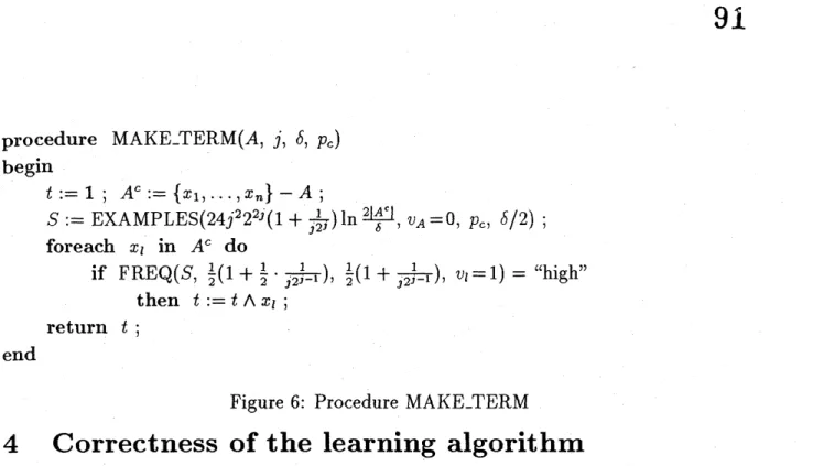
procedure

$MAKE_{-}TERM(A, j, \delta, p_{c})$

begin

$t:=1$ ; $A^{c}$ _{$:=\{x_{1}, \ldots, x_{n}\}-A$} ;

$S:= EXAMPLES(24j^{2}2^{2j}(1+\frac{1}{j2^{j}})\ln\frac{2|A^{c}|}{\delta}, v_{A}=0, p_{c}, 6/2)$ ;

foreach $x_{l}$ in $A^{c}$ do

if FREQ$(S, \frac{1}{2}(1+\frac{1}{2}\cdot\frac{1}{j2J-1}),$ $\frac{1}{2}(1+\frac{1}{j2J-1}),$ $v_{l}=1$) $=$ “high”

then $t:=t\wedge x_{l}$ ;

return $t$ ;

end

Figure 6: Procedure MAKE-TERM

4

Correctness of the

learning algorithm

Many of the statements in this section are involved with Lemma 2.5. As is shown in the remark after the lemma, we simply claim that the fact that FREQ returnes “low” implies $Pr[E(v)]<p$, and that the fact that FREQ returnes “high” implies $Pr[E(v)]>p-\alpha$

without saying the phrase “with highprobability”. Also we simply claim that EXAMPLES produces the desired sequence, omitting the same phrase.

Fact 4.1 $(1- \frac{\delta}{m})^{m}\geq 1-\delta$ for any $m\geq 1,0\leq 6\leq 1$.

Lemma 4.2 Let $f$ be a non-redundunt formula in k-term MDNF and $t$ be any term

in Term$(f)$. Let $v$ be a random positive example of $f$. For any variable $x$; in $Var(t)$,

$Pr[v_{i}=1]\geq\frac{1}{2}$

(

$1+ \frac{1}{2^{k-1}}$ .

P.r

$[t(v)=1]$

).

Proof. Let $T$ be the set of terms $t’$ in Term_$(f)$ such that _{$x_{t}\in Var(t’)$}. Let _$f’$ be

the disjunction of terms in $T$ and $f”$ be the disjunction of terms in Term$(f)-T$. Then,

$Pr[v_{t}=1]=Pr$[$f^{u}(v)=1$ and $v_{i}=1$] $+Pr$[$f”(v)=0$ and $f’(v)=1$]

$\geq\frac{1}{2}$($Pr[f”(v)=1]+Pr[f”(v)=0$ and $f’(v)=1]+Pr[f^{n}(v)=0$ and $t(v)=1]$)

$= \frac{1}{2}$($1+Pr[f”(v)=0$ and $t(v)=1]$).

From Fact 3.1, there exists a set $A$ such that $|A|\leq k-1,$ $A\cap Var(t)=\emptyset$ and that $v_{A}=0$ implies $f”(v)=0$. Therefore, $Pr$[$f”(v)=0$ and $t(v)=1$] $\geq Pr$[$v_{A}=0$ and $t(v)=1$] $= \urcorner^{1}2^{A}\urcorner Pr[t(v)=1]\geq\frac{1}{2^{k-1}}Pr[t(v)=1]$. $\square$

Proposition 4.3 Let $A$ be the set returnd by the procedure _{$SUPPRESS_{-}G(g, i, 6)$}.

Then $Pr[v_{A}=0]>\frac{1}{2}\frac{\epsilon}{i2^{|A|+1}}$

Proof. If the procedure SUPPRESS-G is called by the learning algorithm $L$, it is

guaranteed that $Pr[g(v)=0]>\epsilon/2$. This fact is easily verified from the remark after

92

From $Pr[g(v)=0]>\epsilon/2$ and the fact that there exist at most $i$ terms in Term$(f)$

$-Term(g)$, there exists aterm$t$ in $Te^{r}rm(f)-Term(g)$ such that $Pr$ [$t(v)=1$ and $g(v)=0$]

$> \frac{1}{i}\frac{\epsilon}{2}$ which implies _{$Pr[t(v)=1]>\frac{\epsilon}{2i}$} Therefore, from Fact 3.1 there exists aset $A$ in $A$

such that $A\cap Var(t)=\emptyset$ and $Pr$[$t(v)=1$ and $v_{A}=0$] $> \urcorner^{1}2^{A}\urcorner\frac{\epsilon}{2i}$. Therefore, it follows that $thereexistsFrom|A|\leq k-i,itiseasytoseethat^{>}\frac{64^{\frac{\epsilon}{l2^{|A|+1}k-l}}t2}{\epsilon}\ln^{\bigcup_{\delta}}anAsuchthatPr[v_{A}=0]$

thelength of the sequence $S$produced

by the procedure EXAMPLES in SUPPRESS-G, satisfies the condition (2-1). Therefore, from Lemma 2.5, there exists an $A$ such that the procedure FREQ returns (_$hgh’$ . On the

other hand, if $Pr[v_{A}=0]<\frac{1}{2}$ $\frac{\epsilon}{i2^{|A|+1}}$ holds, the procedure FREQ returns $1_{oW}’$ )

Thus, it is concluded that SUPPRESS-G correctly returnes $A$ such that $Pr[v_{A}=0]>\frac{1}{2}\frac{\epsilon}{i2^{|A|+1}}$ $\square$

Note that all terms in Term$(g)$ are suppressed by the valiables in $A$ which was returnd

by SUPPRESS-G.

Proposition 4.4 Let $p_{c}$ and $A$ be as in the procedure SUPPRESS F. For any $A$ during

the procedure SUPPRESS-F, $Pr[v_{A}=0]\geq p_{c}$.

Proof. From Proposition 4.3, $Pr[v_{A}=0]$ is greater than $p_{c}$ when the procedure

SUP-PRESS-F was called from L.

Now assume that $Pr[v_{A}=0]\geq p_{c}$ at the beginning ofthe while loop for some iteration

step. Let $x_{l}$ be the variable added to $A$ in this iteration step of SUPPRESS-F.

From Proposition 2.4, the procedure EXAMPLES, which is called first in this itera-tion, produces a sequence $S$ composed of $64j \ln\frac{4(i-1)|A^{c}|}{\delta}$ positive examples satisfying the

condition $v_{A}=0$ under the assumption. Each vector in $S$ was drawn uniformly from

the positive examples satisfying $v_{A}=0$. It is easy to see that above length of the

se-quence satisfies the condition (2-1). Thus, from Lemma 2.5, the condition for variables in $V_{1}$ that FREQ$(S, \frac{1}{2}\frac{1}{2j}\frac{1}{2j}v_{l}=0)$ returns “high” imphes $Pr[v_{l}=0|v_{A}=0]>\frac{1}{2}$ $\frac{1}{2_{J}}$

Therefore we have $Pr[v_{A\cup\{x_{I}\}}=0]=Pr$[$v_{l}=0$ and $v_{A}=0$] $=Pr[v_{l}=0|v_{A}=0]\cdot Pr[v_{A}=0]$

$> \frac{1}{2}\frac{1}{2j}\cdot Pr[v_{A}=0]$

.

And $p_{c}$ is set to$p_{c} \cdot\frac{1}{2}\cdot\frac{1}{2_{\dot{J}}}$ whenever $x_{l}$ is added to $A$. Therefore the

assumption is true for the next iteration step.

Thus, the assumption is true for all iteration step, and the proposition follows. $\square$

From Proposition 4.3 and Proposition 4.4, it follows that $Pr[v_{A}=0]=\Omega(\epsilon)$ during the

whole algorithm L. Also note that Proposition 4.4 implies that there always remains at least one term in Term$(f)-Term(g)$ that is not suppressed by the valiables in $A$.

Proposition 4.5 Let $x_{l}$ be the variable added to $A$ in the procedure SUPPRESS-F.

There exists some term in Term$(f)$ that is suppressed by $x_{l}$ but not by the variables in $A$.

Proof. From Proposition 2.4 and Proposition 4.4, the procedure EXAMPLES, which is called second in each iteration, produces a sequence $S$ of$24j^{2}2^{2j} \ln\frac{4(i-1)|A^{c}|}{\delta}$ positive

ex-amples satisfying the condition $v_{A}=0$. The first bound of the condition (2-1) of Lemma

93

for $j\geq 1$

,

and the right most term is equal to the second bound of (2-1). Thus, above length of the sequence satisfies the condition (2-1). Therefore, from Lemma 2.5, the

con-dition for variables in $V_{2}$ that FREQ$(S, \frac{1}{2}\frac{1}{2}(1+\frac{1}{2}\cdot\frac{1}{j2^{j-1}}),$ $v_{l}=1$) returns “high” implies

$Pr[v_{l}=1|v_{A}=0]>1/2$, the proposition follows. $\square$

Lemma 4.6 Let $f$ be a target formulae. The procedure MAKE-TERM called from the

learning algorithm $L$ returns a term in Term$(f)-Term(g)$.

Proof.

Let $j$ and $A$ be those in the procedure MAKE-TERM.

Assume that $j=1$ . From Proposition 4.5, variables in $A$ suppresses $k-1$ terms in

Term$(f)$. Therefore, there remains just one term $t$ not suppressed by variables in $A$.

Therefore, $Pr[v_{l}=1|v_{A}=0]$ is equal to 1 if $x_{l}$ is in $Var(t)$, and 1/2 otherwise. Thus, as

thefollowing argumentshows, the remainingterm$t$ is produced correctly in MAKE-TERM.

Now assume that $j>1$. In this case, the conditions for values returned by FREQ in the procedure SUPPRESS-F are not satisfied: For any variable $x_{l}$ in $A^{c}=\{x_{1}, \ldots, x_{n}\}-A$,

$Pr[v_{l}=0|v_{A}=0]<\frac{1}{2j}$ or $Pr[v_{l}=1|v_{A}=0]<\frac{1}{2}(1+\frac{1}{2}\cdot\frac{1}{j2^{J-1}})$. Since there remain at most $j$ terms not suppressed by the variables in $A$, there exists a term $t$ in Term$(f)$

$-Term(g)$ such that $Pr[t(v)=1|v_{A}=0]>\frac{1}{j}$ Therefore, by Lemma 4.2, $Pr[v_{l}=1|v_{A}=0]$

$> \frac{1}{2}(1+\frac{1}{2^{J-1}}\cdot\frac{1}{\dot{J}})$ for any $x_{l}$in $Var(t)$

.

On the other hand, for any$x_{l}$ in$A^{c}-Var(t)$, we have

$Pr$[$v_{l}=0$ and $t(v)=1|v_{A}=0$] $=Pr$[_{$v_{l}=0|t(v)=1$} and $v_{A}=0$] $\cdot Pr[t(v)=1|v_{A}=0]$ $> \frac{1}{2}$ $\frac{1}{\dot{J}}$ which implies $Pr[v_{l}=0|v_{A}=0]>\frac{1}{2j}$ Therefore, since the first condition for $x_{l}$

chosenin $SUPPRESS\lrcorner$? is satisfied, the second condition is not satisfied: $Pr[v_{l}=1|v_{A}=0]$

$< \frac{1}{2}(1+\frac{1}{2}\cdot\frac{1}{J^{2^{g-1}}})$ for any $x_{l}$ in $A^{c}-Var(t)$.

From Proposition 2.4 and Proposition 4.4, the procedure EXAMPLES, which is called in MAKE-TERM, produces a sequence of $24j^{2}2^{2_{\dot{J}}}(1+ \frac{1}{j2^{j}})\ln\frac{2|A^{c}|}{\delta}$ positive examples

satis-fying the condition $v_{A}=0$. The first bound of the condition (2-1) of Lemma 2.5 becomes

$16j^{2}2^{2j}(1+ \frac{1}{j2^{y-1}})\ln\frac{4(i-1)|A^{c}|}{\delta}$, and the second bound becomes $24j^{2}2^{2j}(1+ \frac{1}{j2^{j}})\ln\frac{4(i-1)|A^{c}|}{\delta}$.

It is easy to see that the second bound is greater than the first one for $j\geq 1$. Thus, above length of the sequence satisfies the condition (2-1). Therefore, from Lemma 2.5, it is concluded that the term$t$ in Term$(f)-Term(g)$ is produced in MAKE-TERM. $\square$

Theorem 4.7 The learning algorithm $L$for k-term MDNF learns k-term MDNF in time

$\mathcal{O}(\frac{n^{k}}{\epsilon}(\ln n+\ln\frac{1}{\delta}))$, using $\mathcal{O}(\frac{1}{\epsilon}(\ln n+\ln\frac{1}{\delta}))$ positive examples.

Proof. Correctness of the algorithm is immediate from Lemma 4.6. All that remain is to estimate the number ofexamples and the time required, and the confidence parameters.

Procedure $SUPPRESS_{-}G(g, i, \delta)$ calls procedure FREQ at most $|A|$ times. Each FREQ

is called with confidence parameter $6/|A|$. Thus, from Fact 4.1, $SUPPRESS_{-}G(g, i, \delta)$ achieves

1–6

confidence.

94

Procedure $SUPPRESS_{-}F(A, i, \delta, p_{c})$ iterates the steps inside the while loop at most

$i-1$ times. In each iteration, procedure EXAMPLES is called twice with confidence

parameter $\delta/4(i-1)$, and procedure FREQ is called $2|A^{c}|$ times with confidence

param-eter $6/4(i-1)|A^{c}|$. Therefore, from Fact 4.1, each iteration has confidence $(1- \frac{\delta}{4(i-1)})^{2}$

. $(1- \frac{\delta}{4(i-1)|A^{c}|})^{2|A^{c}|}\geq(1-\frac{\delta}{2(\cdot-1)})^{2}\geq 1-6/(i-1)$. Therefore, $SUPPRESS_{-}F(A, i, \delta, p_{c})$ achieves $1-\delta$ confidence.

Procedure $MAKE_{-}TERM(A, j)\delta,$ $p_{c}$) calls EXAMPLESoncewith confidence parameter

6/2, and calls FREQ

_I

$A^{c}|$ times with confidence parameter $\delta/2|A^{c}|$. Therefore, the same

argument as above shows that $MAKE_{-}TERM(A, j, \delta, p_{c})$ achieves

1–6

confidence.

Algorithn $L$itselfcalls FREQ at most $k-1$ times with confidence parameter _{$\delta/4(k-1)$},

calls SUPPRESS-G at most $k-1$ times with confidence parameter $\delta/4(k-1)$, calls

SUP-PRESS-F at most $k$ times with confidence parameter $\delta/4k$, and calls MAKE-TERM at

most $k$ times with confidence parameter _$6/4k$. From Fact 4.1, it is concluded that the

whole algorithm $L$ achieves $1-\delta$ confidence.

Procedure EXAMPLES called by $L$ itself calls POS $\mathcal{O}(\frac{1}{\epsilon}\ln\frac{1}{\delta})$ times. From $1\leq i\leq k$

and $|A|\leq n^{k-1}$, EXAMPLES called by SUPPRESS-G calls POS $\mathcal{O}(\frac{1}{\epsilon}(\ln n+\ln\frac{1}{\delta}))$ times.

From $|A^{c}|<n,$ $1\leq i_{J}.j\leq k$ and the fact that $p_{c}=\Omega(\epsilon)$ during the whole algorithm $L$, it is

easy to see that each EXAMPLES called by SUPPRESS-F and MAKE-TERM calls POS

$\mathcal{O}(\frac{1}{e}(\ln n+\ln\frac{1}{\delta}))$ times. Since the numbers of iterations in $L$ and SUPPRESS-F are both

at most $k$, it is concluded that the total number of examples required is $\mathcal{O}(\frac{1}{\epsilon}(\ln n+\ln\frac{1}{\delta}))$ .

When the procedure $SUPPRESS_{-}G(g, i, \delta)$ is called from $L$, at most _{$|A|\leq n^{k-i}$} sets

$A$ must be tested via $\mathcal{O}(\frac{1}{\epsilon}(\ln n+\ln\frac{1}{\delta}))$ positive examples. This part dominates the time

required over the whole algorithm. Therefore, it is easy to see that the total time required is $\mathcal{O}(\frac{n^{k}}{e}(\ln n+\ln\frac{1}{\delta}))$

.

Completed the whole proof of Theorem 4.7. $\square$

5

Learning

k-term MDNF

in

the

presence

of

errors

In this section, we consider the learnability ofk-term MDNF in the presence of noise in the examples, adopting the malicious error model which is introduced in [V85] and studied in [KL].

$POS_{\beta}^{M}(f)$ is an oracle with following features: With probability _$1-\beta$, it behaves the

same as $POS(f)$ and, with probability $\beta$, it produces an arbitrary answer possibly chosen

maliciously by an adversary. $POS_{\beta}^{M}(f)$ is called $POS(f)$ with

malicious

error rate $\beta$, and

simply written as $POS_{\beta}^{M}$ when no confusion arises. Without loss ofgenerality, $0\leq\beta<1/2$

is assumed. Since we are concerned with only positive examples, we do not need to consider

95

in section 2, we have the definition of learnability from $POS_{\beta}^{M}$.

$Pr$[$E(v)$ : POS] denotes the probalility of an event $E(v)$ where $v$ is given by POS, and

$Pr[E(v):POS_{\beta}^{M}]$ denotes the probahlity of the event $E(v)$ where $v$ is given by $POS_{\beta}^{M}$.

Fact 5.1 Let $r,$ $s$ be such that$0\leq r,$ $s\leq 1$. If$Pr$[$E(v)$ : POS] $\geq r$ then$Pr[E(v)$ : $POS_{\beta}^{M}]$

$\geq(1-\beta)r$, and if $Pr$[$E(v)$ : POS] $\leq s$ then $Pr[E(v):POS_{\beta}^{M}]\leq(1-\beta)s+\beta$.

Following lemma is analogous to Lemma 2.5. It tells that the procedure FREQ can be used to estimete the probability of an event in the case of occuring errors as well.

Lemma 5.2 Let $p,$ $\alpha,$

$\delta$ be as in the Lemma 2.5. Let _$S$ be a sequence of

$m$ vectors each of which is given independently by $POS_{\beta}^{M}$, and let _$m$ be such that $m \geq\neq 4\alpha 8\ln\frac{1}{\delta}$. Let $\beta,$ $\beta_{0}$

satisfy the following condition (5-2).

$0\leq\beta\leq\beta_{0}\leq\alpha/4$ (5-2)

Let $p’=$ $(1-\beta_{0})p$ and of $=\alpha-(1+\alpha)\beta_{0}$. If $Pr$[$E(v)$ : POS] $\leq p-\alpha$ then

FREQ($S,$ $p’$ –of, $p’,$ $\delta$) returns “high” with probability at most 6, and if$Pr$ [$E(v)$ : POS]

$\geq p$ then it returns “low” with probabihty at most $\delta$.

Proof. Using Fact 5.1 and an argument analogous to the proof of Lemma 2.5, the lemma can be proved. Details are left to the readers. $\square$

When we attempt to estimete the conditional probability $Pr$[_$E(v)|C(v)$ : POS],

the situation is slightly different. Let $S$ be a sequence of vectors produced by

EXAMPLES(m, $C(v),$ $p_{c},$ $\delta$), where POS is replaced with _{$POS_{\beta}^{M}$} in the procedure

EX-AMPLES. Each vectors in $S$ can be seen as a vector that is produced independently by

an oracle which produces positive examples satisfying the condition $C(v)$ uniformly with

malicious error rate $\beta’$. From the assumption that $Pr$[$C(v)$ : POS] _{$\geq p_{c},$} $\beta<1/2$, and Fact

5.1, it follows that $\beta’=\beta/Pr[C(v):POS_{\beta}^{M}]\leq\beta/(1-\beta)p_{c}<2\beta/p_{c}$

.

Therefore, replacing

$\beta$ with $\beta’$ in Lemma 5.2, we have that if $\beta$ and $\beta_{0}$ satisfy the followong condition (5-3),

then Lemma 5.2 can be used to estimete the conditional probability as well.

$0\leq\beta\leq\beta_{0}\leq\alpha p_{c}/8$ (5-3)

Theorem 5.3 There is aconstant $0<c_{k}<1$ such that k-term MDNF is learnable from

$POS_{\beta}^{M}$ for $\beta=c_{k}\epsilon$

.

Proof. Applying the modification suggested by Lemma 5.2, it is easy to modify the learning algorithm $L$ to the learning algorithm $L^{*}$ that learns k-term MDNF in the

presence oferrors. And it can be seen that in the modified algorithm, right most terms in the condition (5-2) and (5-3) are both $\Omega(\epsilon)$. Thus, Lemma 5.2 and Lemma 4.7 imply the

96

theorem. Details are left to the readers. 口

Acknowledgement

We would like to thank Les Valiant for pointing us [KMP].

References

[GM] Qian Ping GU and Akira Maruoka, “Leaning Monotone Boolean Functions by Uniformly Distributed Examples”, submitted.

[H] D. Haussler, “Quantifying the inductive bias in concept learning”, extended abstract in Proc. AAAI $8\theta$, Philadelphia, PA., 1986, pp.485-489.

[KL] M. Kearns and M. Li, “Learning in the presence of malicious errors”, In

proceedings

_of

the 20th Annual ACM Symposium on Theory

_of

Computing, pp.267-280, 1988.

[KLPV87a] M. Kearns, M. Li, L. Pitt and L. G. Valiant, “Recent Results on Boolean Concept Learning”, Proc.

_4th

Int. Workshop on Machine Learning, Morgan Kaufmann, Los Altos, CA., 1987, pp.337-352.

[KLPV87b] M. Kerns, M. Li, L. Pitt and L. G. Valiant, “On the Learnability of Boolean Formulae”, In proceedings

_of

the 19th Annual ACM Symposium on Theory

_of

Computing, pp.285-295, 1987.

[KMP] L. Kucera, A. Marchetti-Spaccamela and M. Protasi, (On _{the learnabihty of}

DNF formulae”, Lecture Notes in Computer Science, 317:347-361, 1988. [PV] L. Pitt and L. G. Vahant, (Computational hmitations onlearningfrom

exam-ples”, Tech. Rept. TR-05-86, Harvard University, 1986.

[V84] L. G. Valiant, “A theory of the learnable”, Communications

_of

the ACM, 27(11), 1984, pp.1134-42.

[V85] L. G. Vahant, (Learning disjunctions of conjunctions”, Proc. 9th IJCAI, Los