Steady pulse solutions to an RLW equation with instability and dissipation

(1)

Steady pulse

solutions to

an

RLW equation with

instability

and

dissipation

大信田丈志 (OOSHIDA

Takeshi),

Faculty

of

Science

川原琢治

(Takuji Kawahara), Faculty

of Engineering

Kyoto University

Abstract

Propertiesofsteadypulse solutions are investigatednumericallyand analytically

for the regularized-long-wave(RLW) equation including the Kuramoto-Sivashinsky

terms. Both positive and negative pulses with oscillatory or monotone tails are

found to be available depending on the effects ofinstability, dissipation, and “base

line”. The solutions are classified in terms of the two parameters defined by the

ratios of three effects.

1 Introduction

Typical wavephenomena involved in nonlinear dispersivemedia with both instability and

dissipation, such as long waves on liquid films, have been investigated in terms of the

Benney equation [1]

$[\partial_{\iota}+\partial_{x}+\partial 3]x[u+u\partial_{x}u+\alpha\partial_{x}2\partial 4+\beta x]u=0$ $(\alpha>0, \beta>0)$. (1)

Its linear dispersion relation is given by

$\omega=k-k^{3}+i(\alpha k^{2}-\beta k^{4})\equiv{\rm Re}\omega+i{\rm Im}\omega$, (2)

and ${\rm Re}\omega=k-k^{3}\equiv\omega_{\mathrm{K}\mathrm{d}\mathrm{V}}$ is the dispersion ofthe Korteweg-de Vries$(\mathrm{K}\mathrm{d}\mathrm{V})$equation [2].

In some media, however, the dispersion relation is not necessarily approximated by the

$\mathrm{K}\mathrm{d}\mathrm{V}$ term. It would be then interesting to investigate such non-KdV-like dispersion in

comparison with the Benney equation.

In this paper, we take up the following equation

$[\partial_{t}+\partial_{x}-\partial_{t}\partial x2]u+u\partial_{x}u+[\alpha\partial 2\beta\partial x]x=+u04$ (a $>0,$ $\beta>0$). (3)

The first two parts of$\mathrm{e}\mathrm{q}.(3)$ is the Regularized-Long-Wave(RLW) equation [3] [4]

$[\partial_{t}+\partial x-\partial t\partial x2]u+u\partial x=u\mathrm{o}$, (4)

which approximatelygoverns the driftwavesin plasmas [5] [6] orthe void (volumefraction)

waves in a general one-dimensional model oftwo-phase systems [7]. The linear dispersion

relation of the RLW equation is given by

(2)

which is reduced to the $\mathrm{K}\mathrm{d}\mathrm{V}$ dispersion

$\omega_{\mathrm{K}\mathrm{d}\mathrm{V}}$ when expanded for small $k$. The third part

of$\mathrm{e}\mathrm{q}.(3)$ is the Kuramoto-Sivashinsky(KS) termsrepresenting

instability (proportional to

$\alpha)$ and dissipation (proportional to $\beta$) $[8][9]$.

The original Benney equation (1) is known to possess asteady pulse solution thanks

to a _{balance between instability and dissipation [10]. The attempt to} _understand _the

$\mathrm{d}\mathrm{y}\mathrm{n}\mathrm{a}\mathrm{m}\mathrm{i}_{\mathrm{C}}\mathrm{s}$($\mathrm{i}.\mathrm{e}.$, the time evolutions) of solutions to eq.(l) in terms of such soliton-like

pulses weakly interacting with one another was quite successful [11] [12].

Now the question is whether the same treatment is applicable to the case of eq. (3),

i.e., the RLW equation with the KS terms, and to seek what differences arise due to the

change in the linear dispersion term. As the first step to this aim, in this paper, we

explore steady pulse solutions of $\mathrm{e}\mathrm{q}.(3)$.

In

_\S

2, we summarize some existing results for the RLW equation and the Benney

equation. Perturbation solutions and numerical results of steady pulsesolutions aregiven

in

_\S

3. Effect of the boundary conditions at infinity is discussed in

_{\S 4.}

Conclusions are

given in

_{\S 5.}

2 Preliminary Remarks

For convenience oflater discussion we summarize several results for the RLW equation

and the Benney equation.

2.1 RLW

equation

The RLW equation (4) was derived first by Peregrine [3] by means of shallow water

approximation ofan “undular bore” in a canal. As is well known, ananalysis of essentially

the same problem has given birth to the $\mathrm{K}\mathrm{d}\mathrm{V}$ equation [2]; in fact, as

far

as extremely

long waves are concerned, the $RLW$_{equation is} _equivalent _{to the} $KdV$ equation. This is

clear ifwe expand (5) for $k\ll 1$, as $\omega_{\mathrm{R}\mathrm{L}\mathrm{W}}=k(1-k^{2}+k^{4}-\cdots)$, to find the leading two

terms are nothing but $\omega_{KdV}$

.

Another way to show the equivalence between the RLW

equation and the $\mathrm{K}\mathrm{d}\mathrm{V}$ equation is to note that for

unidirectional propagation of long

waves $\partial_{t}u\simeq-\partial_{x}u[4]$.

The RLW equation, however, is different from the $\mathrm{K}\mathrm{d}\mathrm{V}$ equation in the following

points:

1. The propagation speed is finite for short wave components, because it follows from

(5) that

$|\omega_{\mathrm{R}\mathrm{L}\mathrm{W}}/k|=1/(1+k^{2})<+\infty$. (6) In contrast, $\omega_{\mathrm{K}\mathrm{d}\mathrm{V}}/k=1-k^{2}$ goes $\mathrm{t}\mathrm{o}-\infty$ as _{$karrow+\infty$}. It means

that the RLWequation is

a “regularization” of the $\mathrm{K}\mathrm{d}\mathrm{V}$ equation in the sense

that the former is free from the

non-locality ofthelatter; thisis whyBenjamin, Bona and Mahony named $\mathrm{e}\mathrm{q}.(4)$

“Regularized-Long-Wave equation” [4].

2. The RLW equation _{admits two distinct families} _of _the _solitary

_wave

_solutions

characterized by positive or _{negative amplitude. For the boundary conditions} $u(zarrow$

$\pm\infty)=0$, they are provided by

$u_{\mathrm{R}\mathrm{L}\mathrm{W}}=A$

sech2

$[(x-ct)/\lambda]$ _{$(\lambda>0)$}, (7)

$A=A(\lambda)=12/(\lambda 2-4)$, $c=c(\lambda)=\lambda^{2}/(\lambda 2-4)$. (8)

This solution consists of two distinct branches, namely (i) $\mathrm{K}\mathrm{d}\mathrm{V}$ branch

$(\lambda>2,$ _$A>$

$0,$ $c>1)$ and (ii) plasma branch $(0<\lambda<2, A<-3, c<0)$. _When $\lambda$ passes across

(3)

2, the pulse solution (7) suffers discontinuous changes. The branch of negative amplitude

solitarywaves is called “plasma branch”, because the RLW equation is applicableto drift

waves in plasma. In that case, solitary waves with $c<0$, as well as those with positive

velocity, must be observable $[13][14]$.

3. The RLW equation is not invariant under the so called Galilei transform. This

fact leads us to consider “base $\mathrm{l}\mathrm{i}\mathrm{n}\mathrm{e}$”

$(\mathrm{i}.\mathrm{e}., u_{b})$ which defines the boundary conditions by

$u(xarrow\pm\infty)=u_{b}$. Concerning the $\mathrm{K}\mathrm{d}\mathrm{V}$ equation, the boundary value problem with

arbitrary $u_{b}$ is reduced to the zero-boundary value case by means of the so called Galilei

transform:

$u(x, t)=u_{b}+v(x’,t’)$, $x=x’+u_{b}t’$, $t=t’$_, ₍₉₎

so that a solution $v$ solved under the boundary conditions $v(x’arrow\pm\infty)=0$ can provide

a solution $u$ under non-zero boundary conditions. However, such Galilei invariance does

not hold for the RLW equation. Instead, the following rescaling

$u=u_{b}+(1+u_{b})\tilde{u}$, $x=\pm\tilde{x}$ $(u_{b<}>-1)$, $t=t^{\sim}/|1+u_{b}|$ (10)

canbeusedto reduce the problem tothecase ofzeroboundaryconditions $(u(xarrow\pm\infty)=$

$0)$ conserving the form of (4) when $u_{b}\neq-1$.

4. The RLW equation isnot completely integrable and seems tobenotsolvable bythe

inverse scattering method, since it admits only several numbers of conserved quantities.

This fact indicates that the solitary waves given by (7) are not ‘soliton’ in an exact sense

but they suffer changes in collisions [14].

For $u_{b}\neq-1$, solitary wave solutions are given by

$u_{\mathrm{R}\mathrm{L}\mathrm{W}}=u_{b}+A$

sech2

$[(x-ct)/\lambda]$ $(\lambda>0)$, (11)

$A=A(\lambda)=12(u_{b}+1)/(\lambda^{2}-4)$_, $c=c(\lambda)=\lambda^{2}(u_{b}+1)/(\lambda^{2}-4)$. (12)

For $u_{b}=-1$ we put $u(x, t)=-1+v(x, t)$, then $v$ satisfies the Equal-Width equation

$[1-\partial_{x}^{2}]\partial_{t}u+u\partial_{x}u=0$. (13)

A steady pulse solution to this equation is given by

$u=3c$

sech2

$[(x-ct)/2]$ $(u(zarrow\pm\infty)=0)$, (14)

and its “width” (characteristic length) remains constant for various values of $c$. This

solution can readily be obtained from (11) by setting $u_{b}arrow-1$ and $\lambdaarrow 2$, i.e., $A$ and $c$

can become finite for $u_{b}=-1$ only if $\lambda=2$.

2.2 Steady

solutions

of the Benney

equation

While the solitary wave solution to the $\mathrm{K}\mathrm{d}\mathrm{V}$ equation contains one arbitrary parameter,

the Benney equation does not allow such a freedom [10]. When the KS terin$\mathrm{s}$ are added

as small perturbations to the $\mathrm{K}\mathrm{d}\mathrm{V}$ equation, then a pulse which propagates in constant

form and speed under the $\mathrm{K}\mathrm{d}\mathrm{V}$ dynamics must generally grow or shrink unless the effect

of perturbation balances each other and determines a special value for the parameter

$\lambda$ signifying the pulse width. Therefore a steady pulse solution of the Benney equation

bearsa definite amplitude, formand velocity corresponding to eachfixedsetofthe control

parameters.

A parallel argument suggests that one-parameterset ofthe steady pulses of the RLW

(4)

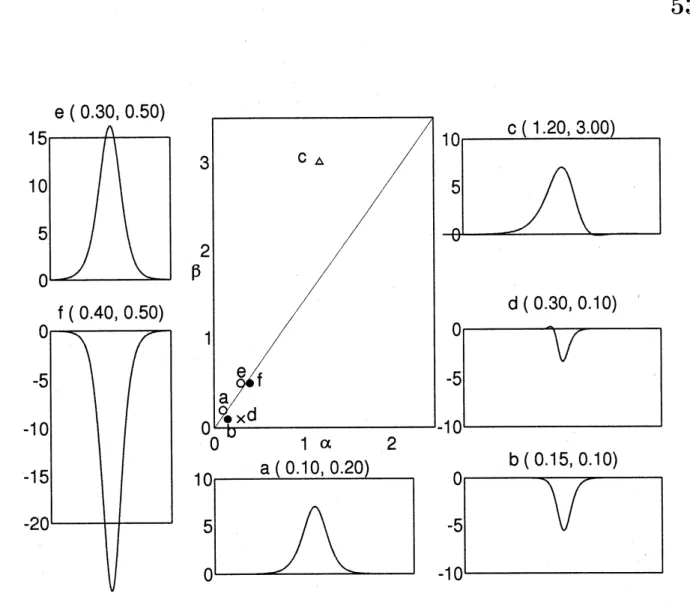
$\mathrm{I}\mathrm{o}\mathrm{g}10\alpha$

Figure 1: The range of$(\alpha, \beta)$ for numerical exploration of steady pulses: _{$\rho=\beta/\alpha,$} _{$u_{b}=0$}.

Symbolsstand for: $\circ$ and $\bullet$, positive and negative pulses with monotonetails; and $\triangle$ and

$\cross$, positive and negative ones with oscillatory tails, respectively.

terms. Perturbationand numerical analyses done in the sequel supportthis suggestion,

as

long as the relative effect of the KS terms is not very large. When that effect amplified,

pulses _{with oscillatory tails resembling those of the KS equation appear. As will be}

shown, two pulses (either positiveor negative amplitude) are possible for the same set of

the parameter values.

To explore such steady solutions, we put $u=u(z),$ _$z=x-ct$ _in $\mathrm{e}\mathrm{q}.(3)$ leading to the

fourth-order ordinarydifferential equation,

$[(1-C)\partial z+c\partial_{z}3]u+u\partial zu+[\alpha\partial 2+\beta zz\partial^{4}]u=0$ _{$(\alpha>0, \beta>0)$}, (15)

ofthe same form as _{for the Benney equation (1). Then the form and the amplitude of}

the equilibrium pulse and the velocity $c$ must be determined at the same time, if the two

parameters $(\alpha, \beta)$ and the “base line” _{$u_{b}=u(zarrow\pm\infty)$} areassigned. Then two questions,

i.e., (i). How the solutions depend on $(\alpha, \beta)$? and (ii). How the solutions depend on

$u_{b}$?

are posed. Nowwe investigate these two points by numerical and mathematical methods.

3 Dependence

of pulse

solutions

on

$(\alpha, \beta)$

In this sectionwe focus our attention to find how a pulse solution of $\mathrm{e}\mathrm{q}.(15)(\mathrm{S}\mathrm{t}\mathrm{e}\mathrm{a}\mathrm{d}\mathrm{y}$ pulse

solution of $\mathrm{e}\mathrm{q}.(3))$ depends on the values of $\alpha$ (instability) and $\beta$ (dissipation).

3.1 Approximation from the

RLW

equation

First, we consider the case when the effect of the KS terms is small and deal with $\mathrm{e}\mathrm{q}.(3)$

as the RLW equation with perturbation by rewriting as

$[\partial_{t}+\partial_{xt}-\partial\partial 2]x\hat{\Pi}u+u\partial_{x}u=\epsilon u$, $\hat{\Pi}\equiv-[\alpha’\partial_{x}^{2}+\beta’\partial_{x}^{4}]$, (16)

where $(\alpha, \beta)\equiv\epsilon(\alpha’, \beta’)$, so that _{$\alpha’\sim\beta’\sim O(1)$}.

(5)

Figure 2: Pulse solutions of the equation (15), numerically obtained for the parameter

values indicated in the graph at the center (andfor $u_{b}=0$). $(\mathrm{a}),(\mathrm{c}),(\mathrm{e})$ arepositive pulses,

while $(\mathrm{b}),(\mathrm{d}),(\mathrm{f})$ are negative. (c) and (d) have an oscillatory tail. The line $(\beta/\alpha=7/5)$

on the parameter plane is predicted by (22) to divide the territories of the positive and

negative pulses. Symbols are the same as in Fig. 1.

The effectofperturbation is tractablebymeansofthe method

_{of modified}

conservation

laws [10] [16]. We utilize the fact that the RLW equation conserves the following three

quantities:

$M= \int u_{0}dx$, $P= \int[u_{0}^{2}/2+(\partial_{x}u_{0)^{2}}/2]dx,$ $H= \int(u_{0}^{3}/6+u_{0}^{2}/2)dx$, (17)

where $u_{0}$ denotes a solution of the RLW equation (4). In the perturbed equation (16), $P$

and $H$ are no more conserved quantities and their changes are expressed by

$dP/dT= \int u\hat{\Pi}udx$, $dH/dT= \int(u+u^{2}/2-u_{xt})\hat{\Pi}udx$, (18)

where $T\equiv\epsilon t$ denotes a slowlyvarying time. Note that $(u+ \frac{1}{2}u^{2}-u_{xt})$ can be equated to

$-\partial_{x}^{-1}\partial_{t}u$ plus some correction oforder $\epsilon$.

We suppose that the zeroth-ordersolution to $\mathrm{e}\mathrm{q}.(16)$has the solutionof theform (11).

Assuming that the parameter $\lambda$ changes slowly with respect to time (i.e., _{$\lambda=\lambda(T)$}) and

substituting (11) into (18), we obtain

(6)

For a steady pulse, the instability$(\alpha)$ and the $\mathrm{d}\mathrm{i}\mathrm{s}\mathrm{s}\mathrm{i}_{\mathrm{P}}\mathrm{a}\mathrm{t}\mathrm{i}\mathrm{o}\mathrm{n}(\beta)$in (19) must be balanced and

from $dP/dT=0$ we obtain

$\lambda^{2}=\lambda_{e}^{2}\equiv 20\beta/7\alpha=20\rho/7$ $(\rho\equiv\beta/\alpha)$, (20)

where the subscript $e$ stands for the equilibrium. Then the equilibrium solution is given

by

$u_{e}=u_{b}+A_{e}\mathrm{s}\mathrm{e}\mathrm{c}\mathrm{h}2[(X-c_{e}t)/\lambda_{e}]$, (21)

$A=A_{e}\equiv 21(u_{b}+1)/(5\rho-7)$, $c=c_{e}\equiv 5\rho(u_{b}+1)/(5\rho-7)$. (22)

(Adoption of$H$ instead of$P$ simply duplicatesthe result.) Thus $\lambda_{e},$ $A_{e}$ and $c_{e}$ depend on

$\rho$ and $u_{b}$. Note that $\rho$ is the ratio of $(\alpha, \beta)$. Perturbation expansion of$\mathrm{e}\mathrm{q}.(15)$ shown in

Appendix A yields the same result in the lowest order of approximation.

The results of the approximation for small $\alpha$ and $\beta$are summed up as follows when we

consider thecase $u_{b}=0$. The equilibrium pulse is characterized in the lowest order solely

by the ratio $\rho--\beta/\alpha$. Hence the amplitude and the velocity are changed discontinuously

$(+\inftyarrow-\infty)$ when $\rho$ is changed continuously passing across 7/5 $(7/5+0arrow 7/5-0)$.

Intuitivelythis is a consequence ofthe equilibrium

$\alpha\partial_{x}^{2}u\sim\beta\partial^{4}xu$, (23)

which defines a representative wave length $\lambda_{0}\sim(\beta/\alpha)^{1/2}$ (now its measure is the width

of the pulse), and of those relations between $\lambda,$ $A$ and $c$ inherited from the RLW pulses

which incorporate discontinuity of the amplitude and the velocity at $\lambda=2$. Thus ajump

of$u\simeq U_{RLW}|_{\lambda=\lambda 0}$ takes place when $\rho$ passes a certain value $\rho_{c}$, such that $\lambda_{0}(p_{C})=2$ and

the above-mentioned result (20) indicates $\rho_{c}=7/5$. It follows from the higher order of

approximation given by $\mathrm{e}\mathrm{q}.(33)$ in Appendix A that the odd part of$u$ suffers a correction

proportional to $\epsilon\sim(\alpha, \beta)$, but the velocity and the even part of $u$ (and therefore the

amplitude) are independent of$\epsilon$ to the first order ofapproximation.

3.2 Numerical calculation of

steady

solutions

Equation (15) wasnumericallysolvedasa nonlinear eigenvalue problem with eigenfunction

$u$ and eigenvalue $c$ under the boundary conditions $u(zarrow\pm\infty)=0$ for various values

of $(\alpha, \beta)$ shown in Fig. 1. The numerical method is explained in Appendix B. As is

illustrated in Figure 2, we distinguish positive and negative pulses according to their sign

of the amplitude, and distinguish the pulses by their tails, calling them monotone or

oscillatory when the eigenequation (36) possesses three real roots or one real and two

complex conjugate ones.

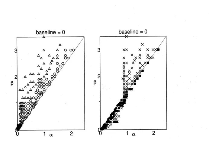
For small values of $\alpha$ and $\beta$, Fig. 3 supports the result of the approximation that

the line $\beta-(7/5)\alpha=0$ on the parameter plane divides regions for the positive and the

negative pulses (the positive ones are situated on the $\beta$-axis side). It turns out that we

can extend this dividing line beyond the limitation $\alpha\sim\beta\ll 1$, so that it still divides

the positive and the negative pulses even for the values of $\alpha$ and $\beta$ as large as 5, as

far as the pulses with monotone tails are concerned. It is natural that the result of the

approximation is not valid for the pulses with oscillatorytails. The invasion of negative,

oscillatory-tailed pulses across the dividing line means that for relatively large values of

$\alpha$ and $\beta$ two distinct pulses are possible, namely a positive and a negative one, when

$p>7/5$ (it is not certain whether such $\rho$ has an upper limit). Invasion of positive pulses

with oscillatory tails into the region of negative pulses was not observed.

(7)

Figure 3: The range ofthe parameters $(\alpha, \beta)$ for which positive (left figure) or negative

(right figure) steady pulses were found $(u_{b}=0)$. Symbols are the same as in Fig. 1.

The prediction of the perturbation approximation (i.e., the relations (22)) are proved

by Fig. 4 for small and not very large values of$\alpha$ and $\beta$. Only negative, oscillatory-tailed

pulses are found not to obey the relations.

Figure 5 shows deviation of the amplitude from (22) for increased value of $\alpha$ and

$\beta$, with $p=2$ fixed. While $\alpha$ and $\beta$ are small, the deviation is of $O(\alpha^{2})(\mathrm{i}.\mathrm{e}.,(22)$ is

almost exact); when $(\alpha, \beta)arrow\infty$ with $\rho=\mathrm{c}\mathrm{o}\mathrm{n}\mathrm{s}\mathrm{t}.(>7/5)$, then, in contrast, the amplitude

grows asymptotically as $O(\alpha)$. (The velocity behaves similarly.) Intuitive interpretation

is that when the KS terms are very large, then the nonlinear term $u^{2}/2$ must participate

in the detailed balance among the terms, which postulates that the amplitude should

be proportional to $\alpha$. In the following section we will show that this situation can be

identified with the case of$u_{b}arrow-1$ and that in this limit $A\propto\alpha$ in fact.

4 Dependence of pulse solutions

on

base

line

Wemean bythe word “base line” the asymptote of the pulse defined by$u_{b}=u(zarrow\pm\infty)$.

In contrast to the case of the original Benney equation, the dependence on $u_{b}$ in not a

trivial problem for $\mathrm{e}\mathrm{q}.(3)$, because it lacks invariance under the Galilei transform.

Now we introduce the rescaling

$u=u_{b}+(1+u_{b})\tilde{u}$, $x=\pm\tilde{x}$ $(u_{b<}>-1)$,

$t=t\sim/|1+u_{b}|$, $(\alpha, \beta)=|1+u_{b}|(\tilde{\alpha},\tilde{\beta})$. (24)

into a problem for $u$ with arbitrary $u_{b}$

(8)

$\Delta$

Figure 4: Dependence of$A$ and $c$ on $\rho=\beta/\alpha$, in the case when $\alpha$ and $\beta$ are not very

large.

Then $\mathrm{e}\mathrm{q}.(25)$ is reduced to a problem for $\tilde{u}$ with zero-leveled $\mathrm{b}\mathrm{a}s\mathrm{e}$ line

$[ \partial_{\overline{t}}+\partial_{\overline{x}}-\partial_{t}^{\wedge}\partial_{\tilde{x}}^{2}]\tilde{u}+\tilde{u}\partial_{\tilde{x}}\tilde{u}+[\tilde{\alpha}\partial_{\tilde{x}}^{2}+\tilde{\beta}\partial\frac{4}{x}]\tilde{u}=0$ _{$(\tilde{u}(\tilde{x}arrow\pm\infty)=0)$}. (26)

The transform (24) tells that the multiplication of $(1+u_{b})$ by $1/k$ is equivalent to

that of $(\alpha, \beta)$ by $k$, taking notice of the tilded variables in (24). In particular, _{$u_{b}arrow-1$}

and $(\alpha, \beta)arrow\infty$ have the same effect $(\tilde{\alpha},\tilde{\beta})arrow\infty$. This similarity law suggests that we

should take $b=(1+u_{b})/\alpha$ and $\rho=\beta/\alpha$ as control parameters, rather than $\alpha,$ $\beta$ and $u_{b}$.

According to this idea we normalize the boundary value problem (25) as follows

$[\partial_{T}-\partial\tau\partial^{2}\mathrm{x}+\partial_{X}^{2}+p\partial_{X}^{4}]U+U\partial_{X}U=0$ _{$(U(xarrow\pm\infty)=b)$}, (27)

where $U=(1+u)/\alpha,$ $T=\alpha t$ and $X=x$.

Now

we

ask whetherasteady solutionexistsfor$u_{b}arrow-1$? Thetransform(24) together

with (22) lead toan inference that when $u_{b}$ goes to-l, then apulse must disappear. This

conjecture turns out to be incorrect. As is mentioned above, $\tilde{\alpha}$ and $\tilde{\beta}$ goes to

$\infty$, which

makes (22) cease to be valid. Numerical calculations prove that for $u_{b}=-1$, when

$\rho>7/5$, steady pulsesolutions indeed exist. Thisis consistent with the divergence of the

$\mathrm{a}\mathrm{m}\mathrm{p}\mathrm{l}\mathrm{i}\mathrm{t}\mathrm{u}\mathrm{d}\mathrm{e}\sim O(\alpha)$shown in Fig. 5. In fact, a transform

$u=\sqrt{\alpha^{3}/\beta}v-1$, $t=(\beta/\alpha^{2})\mathcal{T}$, $x=\sqrt{\beta/\alpha}\xi$, (28)

rewrites $\mathrm{e}\mathrm{q}.(3)$ into the KS equation with the RLW-like dispersion termas aperturbation,

$[ \partial_{\tau}+\partial 2+\xi\partial 4]\xi-\frac{1}{\rho}\partial \mathcal{T}\partial_{\xi}^{2}v+v\partial_{\xi}vv=0$, (29)

where a steady pulse solution is possible for relatively large values of $\rho$. As is noted at

the end of

\S

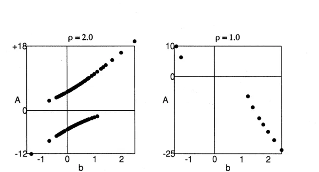
3, the transform (28) shows that $A= \max|u+1|$ is proportional to $\alpha$.

From the point of view of the normalized equation (27), the existence of pulses for

$u_{b}=-1$ indicates that the curve of the relation between the amplitude $A$ (relative to the

(9)

$\mathrm{p}=\beta/a=2.0$

Figure 5: Deviation of $A$ from (22), shown against $\alpha$ in log-log plot; $p=\beta/\alpha=2.0$ is

fixed.

base line) and the level of the base line $b$deviatesfrom the line going through the original

point (Fig. 6.1). The symmetry of Fig. 6.1 with respect to the origin is a manifestation

of the invariance of (27) under the reflection

$Uarrow-U$_, $Xarrow-X$_, $Tarrow T$, (30)

with $b$ replaced $\mathrm{b}\mathrm{y}-b$. Particularly, when $b=0$ (i.e., $u_{b}=-1$), the whole problem (27)

is symmetric with respect to the reflection, i.e., pulses with either sign can exist quite

equally. The observed fact that two different pulses are possible for a certain range of

$(\alpha, \beta)$ when $u_{b}=0$ corresponds to the double-valuedness of$A=A(b)$ in Fig. 6.1. This

figure suggests that either of the two solutions can be continuously deformed to the other,

changingthecontrolparameters (inclusive of$u_{b}$) andjust oncereflecting the solutionwith

respect to some point onthe line $u_{b}=-1$.

Figure 6.2 suggests, on the other hand, that if$\rho=1.0<7/5$ a pulse solution cannot

exist for $b=0$. A transform $u=\sqrt{\frac{\alpha^{2}}{\beta}}w-1$ yields an equation

$\partial_{\tau}[1-\partial_{x}^{2}]w+w\partial_{x}w+\rho\partial_{x}2+w\rho\partial_{x}24w=0$ _{$(w(xarrow\pm\infty)=0)$}. (31)

For small$\rho$ it is the Equal-Width equation (13) perturbed by the KS terms. An analysis

similar to that for $\mathrm{e}\mathrm{q}.(3)$ reveals that no equilibrium pulse is possible (unless

$\rho=7/5$),

because the “wave length” of the pulses (14) cannot be changed.

5 Conclusion

In terms of the perturbation approximation and the direct numerical calculation, we

explored how the steady travelling pulse solutions of $\mathrm{e}\mathrm{q}.(3)$ depend on $(\alpha, \beta)$ and $u_{b}$.

(10)

Figure6: Dependence oftheamplitude $A$on$b$inthenormalizedequation (27), for

$\rho=2.0$

(left figure) and for $\rho=1.0$ (right figure).

1. The balance between instability and dissipation decides the representative length

$\lambda\sim\sqrt{\beta/\alpha}$, just like in the original Benney equation. When the pulse is sech-like

with monotone tails, it can bear only afixed amplitude and a velocityowing to the

dependence of the amplitude and the velocity on $\lambda$. In particular,

$\rho>7/5$ stands

for positive equilibrium amplitude and $\rho<7/5$ negative one.

2. The level of the base line, $u_{b}$, has a non-trivial meaning. It is not the simple

magnitude of$\alpha(\sim\beta)$ but the magnitude of$b=(1+u_{b})/\alpha$ that decides the relative

importance of the KS terms, i.e. whether the pulse is more RLW-like than $\mathrm{K}\mathrm{d}\mathrm{V}$-like

or not. When $u_{b}\sim-1$, the solutions are not RLW-like even for small $(\alpha, \beta)$ but

rather $\mathrm{K}\mathrm{S}$-like as characterized by oscillatory tails and by the

possibility of both

signs for the same control parameters.

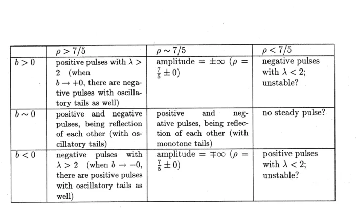
In Table 1, the features ofthe pulsesin variouscases are summarized accordingto the

values of$\rho=\beta/\alpha$ and _{$b=(1+u_{b})/\alpha$}.

We hope that the dynamics of$\mathrm{e}\mathrm{q}.(3)$ can be described to some extent in terms ofthe

soliton-like pulses weaklyinteracting one another. The results of this study suggest that

the “base line” (or probably its local level), or an extremely long wave structure, must

take part in such description of dynamics as well as the pulses with $\lambda\sim(\beta/\alpha)^{1/2}$, because

the displacement of the base line, probably even locally, changes the character of the

equilibrium pulse. In otherwords, when (positive) pulses growfrom small buds collecting

and incorporating the “mass” $u$ (conserved under the evolution equation with a form

$u_{t}+J_{x}=0)$, then they lower the “environmental” level of $u$, i.e., changes the uniform

background on which the pulses exist. Our result says that this change influences the

pulses in return. A lack ofthe Galilei invariance in $\mathrm{e}\mathrm{q}.(3)$ expresses such back influence

fromthe environment to the pulses, which may reflect one aspect of the reality in some

physical systems.

(11)

Table 1: Classification of steady travelling pulses in terms of$p=\beta/\alpha$ and $b=(1+u_{b})/\alpha$.

A

Calculation

of

an

equilibrium

pulse by

perturba-tion

We solve$\mathrm{e}\mathrm{q}.(16)$ bymeans ofastandard perturbation expansion [12]. Under the boundary

conditions $u(zarrow\pm\infty)=0,$ (16) is once integrated for the steady case, into which we

substitute the following expansion:

$u=u^{(0)(1)(2)}+\epsilon u+\epsilon^{2}u+\cdots$, $c=c+(0)\epsilon C(1)+\epsilon^{2()}C2+\cdots$

.

(32)

When we adopt the sech-pulse (7) for $O(\epsilon^{0})$-equation, the solvability condition for $u^{(1)}$

gives $\lambda^{2}=(20/7)\rho$, which then decides $u^{(0)}$ and $c^{(0)}$. This result coincides with that

obtained by the modified conservation laws. From the solvability of $O(\epsilon^{2})$-equation on

$u^{(2)}$ we find $c^{(1)}=0$

.

Now $O(\epsilon^{1})$-equation is aninhomogeneous linear equation on asingle

unknown function $u^{(1)}$, whose solution under the restriction _{$(d/dz)^{2}u^{()}1=0$} is given by

$u^{(1)}=u^{(1)}( \rho;z)=\frac{36\alpha’}{5\lambda}\mathrm{s}\mathrm{e}\mathrm{c}\mathrm{h}^{2}\frac{z}{\lambda}\tanh\frac{z}{\lambda}\ln[\mathrm{s}\mathrm{e}\mathrm{c}\mathrm{h}^{2_{\frac{z}{\lambda}]}}$ $( \lambda^{2}=\frac{20}{7}\rho)$ , (33)

which turns out to be an odd (anti-symmetric) function of$z$.

$\mathrm{B}$

Numerical method

to

calculate steady pulses

Supposing $u_{b}=u(zarrow\pm\infty)$ is given, we once integrate $\mathrm{e}\mathrm{q}.(15)$ and rewrite the result in

a matrixform:

$\frac{d}{dz}=-$

,

(34)

where $u’=u-u_{b}$ and

(12)

The set of equations (34), regarded as a dynamical system with $z$ as the time, has

fixed points ${}^{t}(0,0, \mathrm{o})$ and _{${}^{t}(0,0, -2(ub+1-c))$}. A pulse solution of

$\mathrm{e}\mathrm{q}.(15)$ corresponds

to a homoclinic trajectory starting from ${}^{t}(\mathrm{o}, 0, \mathrm{o})$. The direction of the stable manifold

and the unstable manifold is given as ${}^{t}(1, \mu, \mu^{2})$ by the roots ofthe eigenequation of the

matrix in (34), namely

$\beta\mu^{3}+c\mu+\alpha\mu+1+ub2=-c\mathrm{o}$_. ₍₃₆₎

Here $u$ behaves like _{$u_{b}+\exp(\mu z)$} when _{$zarrow\pm\infty$}. The

essence

of the calculation is

to integrate numerically the set of$\mathrm{e}\mathrm{q}\mathrm{s}.(34)$ along the one-dimensional

unstable manifold

(which depends on $c$), and to seek such value of_$c$ that the trajectory will return

(along

the stable manifold) to the original point as precisely as possible. _{This is known as the}

shooting method [15] [16].

References

[1] D. J. Benney: J. Math. Phys. 45, 150 (1957)

[2] D. J. Korteweg&G. de Vries: Phil. Mag. (v), 39, 422 (1895)

[3] D. H. Peregrine: J. Fluid Mech. 25, 321 (1966)

[4] T. B. Benjamin, J. L.

Bona&J.

J. Mahony: Phil. Trans. R. Soc. London, A272, 47

(1972)

[5] V. I. Petviashvili: Sov. J. Plasma Phys. 3, 150 (1977) (English translation)

[6] J. D.

Meiss&W.

Horton: Phys. Fluids 25,

1838

(1982)

[7] T. Kawahara: IUTAM Symposium on “Waves in $\mathrm{l}\mathrm{i}\mathrm{q}\mathrm{u}\mathrm{i}\mathrm{d}/\mathrm{g}\mathrm{a}\mathrm{s}$ and

$1\mathrm{i}\mathrm{q}\mathrm{u}\mathrm{i}\mathrm{d}/\mathrm{V}\mathrm{a}\mathrm{P}^{\mathrm{o}\mathrm{r}}$

two-phase system”(1994)

[8] Y.

Kuramoto&T.

Tsuzuki: Prog. Theor. Phys. 55,

356

(1976)

[9] G. I. Sivashinsky: Acta Astronautica4, 1177 (1977)

[10] T. Kawahara: Phys. Rev. Lett. 51, 381 $(1983)/$

[11] T.

_Kawahara&S.

_{Toh: Phys.} _Fluids _31,

₂₁₀₃

₍₁₉₈₈₎

[12] _{S. Toh&T. Kawahara:} _{J. Phys.} _Soc. _{Jpn. 54,} ₁₂₅₇ ₍₁₉₈₅₎

[13] J. D. Meiss: in_{W.Horton, Jr&L.}“Statistical Physics and Chaos in Fusion Plasmas” ed. by C.

E. Reichl, John Wiley&Sons, 273 (1984)

[14] P. J. Morrison, J. D. Meiss&J. R. Cary: Physica 11D, 324 (1984)

[15] S. Toh: J. Phys. Soc. Jpn. 56, 949 (1987)

[16] T. _{Kawahara: “Soriton}_kara_Kaosu _e”, _Asakura _{Shoten, Tokyo (1993)} _{(in Japanese)}