Flow induced around a sphere with a nonuniform surface temperature in a rarefied gas, with application to the drag and thermal force problems ofa spherical particle
with an arbitrary thermal conductivity
S. TAKATA and Y. SONE
京大工航空宇宙 高田 滋, 曾根 良夫
Division ofAeronautics and Astronautics, GraduateSchool of Engineering, Kyoto University, Kyoto 606-01, Japan.
Abstract
A flow induced around a sphere with a nonuniform surface temperature in a rarefiedgas
is investigated on the basis of the linearized Boltzmann equation for hard-sphere molecules
and diffusereflection condition. With the aid of theaccurate and efficient numerical method
developed by the authors with Aoki [S. Takata, Y. Sone, and K. Aoki, Phys. Fluids $A,$ $5$,
716 (1993)$]$, the behavior of the gas, the velocity distribution function as well as macroscopic
variables and force on the sphere, is clarified for the whole rangeof the Knudsen number. In
addition, thesolutions of the drag and thermal force (thermophoresis) problems ofaspherical
particle with an arbitrary thermal conductivity are obtained by appropriate superpositions of
the present solution and thoseofasphere with infinite thermal conductivity, obtained bythe
authors withAoki. The result of the thermal force is compared with various experimental data.
I. Introduction
Gasdynamicsproblemsinasmallsystem,aswellas those ofararefiedgas, whichareimportant in aerosol science and micromachine engineering, require kinetic theory analysis, since the mean
freepath is comparable to the small characteristic length of the system. Whenthe kinetic effector
the effectof rarefaction ofa gasis important, thetemperaturefield and solid walls, thoughat rest, have important effects on gas motion. For small Knudsen numbers, according to the asymptotic
$\mathrm{t}\mathrm{h}\mathrm{e}\mathrm{o}\mathrm{r}\mathrm{y}^{1-5}$, developed by a systematic analysis of the Boltzmann equation, the temperature and
wall effectson gasmotion, suchas thermalcreep $\mathrm{f}\mathrm{l}\mathrm{o}\mathrm{w}^{6}-8$
, thermal stress slip$\mathrm{f}\mathrm{l}\mathrm{o}\mathrm{w}^{9}’ 10$, and nonlinear
thermal stress
flow11
, are characterized by the local behavior of the system. For intermediate andlargeKnudsen numbers, these effects are not characterized only by the local behavior, suchas the
temperaturegradient of the wall in the thermalcreepflow, and globalgeometryof thesystemis also
important. Thus, analyses of various typical systems are useful for general understanding. In the presentpaper we take the systemwhere aspherewith anonuniform surfacetemperature is placed ina unifomgasat rest, and investigate the behavior of thegas, especiallythe flow induced around the sphere and the force on the sphere, for the whole rangeofthe Knudsen number on the basis ofthe standard Boltzmann equation for hard-sphere molecules. The numerical method adopted in the analysis is a combination of the hybrid-finite-difference method, capable of describing the discontinuity of the velocity distribution function in thegas, and the numerical kernel method, an
efficient method of computation of the collision integral, in Ref. 12.
The problem has important applications to analyses of the drag and thermal force problems ofa spherical particle with an arbitrary thermal conductivity. The drag problem (Problem $\mathrm{D}$, for
short) is concerned withaparticlein auniform flow ofa gas, and the thermal force (thermophore-sis) problem (Problem $\mathrm{T}$, for short) is concerned with a particle in a gas at rest with a uniform
temperature gradient. These problems, important in aerosol science, have been studied by various authors (e.g., Refs. 13-27, 12 for problem $\mathrm{D}$; Refs. 28-35, 9, 36-44, 10, 45-47 for problem $\mathrm{T}$; and
Refs.
48-53
for both problems). It is, however,recent that the problems areanalyzed accurately forthe wholerange of the Knudsen number on the basis of the standard Boltzmann equation. That is, in Refs. 12 and 47, the problems $\mathrm{D}$ and $\mathrm{T}$ for a sphere with a uniform surface temperature
areanalyzed numerically on the basis of the Boltzmannequation for hard-sphere molecules. The results apply only to the drag and thermal force problems for a spherical particle with infinite
thermalconductivity. The dragor thermal force problem fora spherical particle with an arbitrary
thermal conductivity, as will be shown in Sec. VI, can be decomposed into two problems: prob-lem $\mathrm{D}$ or $\mathrm{T}$ for a sphere with a uniform surface temperature and the problem ofa sphere with a
nonuniform temperature, and the solution is obtained as an appropriatesuperposition ofthe two
problems. This is another
reason
that we consider the problem ofa sphere with a nonuniformsurface temperature in this paper. II. Problem and notations
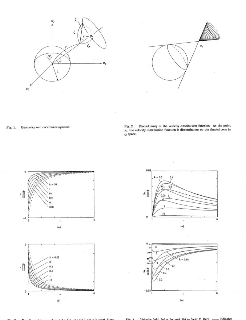
In Secs. III-V, we consider a spherical body with a nonuniform surface temperature [radius
$\mathrm{L}$ and surface temperature $\mathrm{T}_{w}=\mathrm{T}_{0}(1+\alpha \mathrm{X}_{1}/\mathrm{L})$, where $\mathrm{X}_{i}$ is a Cartesian coordinate system with
its origin at the center of the sphere and $\alpha$ is aconstant] in a rarefied gas at rest (pressure$p_{0}$ and
temperature $\mathrm{T}_{0}$), and investigate the steady flow induced around the sphere and the force on the
sphere under the following assumptions:
(i) The gas molecules are hard spheres of a uniform size and undergo complete elastic collisions between themselves.
(ii) Thegasmolecules are reflected diffuselyon the sphere.
(iii) Themagnitude of the temperature variation $\alpha$ is sosmall that the equation and the boundary
condition can be linearized around the uniform equilibrium state at rest with pressure $p_{0}$ and
temperature $T_{0}$.
Then, in Sec. VI weconsider the drag and thermal force problems for a spherical particle with an
arbitrary thermal conductivity.
We summarize other main notations used in this paper: $p_{0}=p_{0}/\mathrm{R}\mathrm{T}_{0;}\mathrm{R}$ (the specific gas
constant) is defined by the Boltzmann constant divided by themassof the molecule; $\ell_{0}$ is themean
free path of the gas molecules at the equilibrium state at rest with pressure $p_{0}$ and temperature
$\mathrm{T}_{0}$ [for a hard-sphere molecular gas, $\ell_{0}=(\sqrt{2}\pi\sigma^{2}\rho 0/m)^{-1}$, where $\sigma$ and $m$ are, respectively, the
diameter and mass of the molecule]; Kn $=\ell_{0}/\mathrm{L}$ (Knudsen number); $k–(\sqrt{\pi}/2)\mathrm{K}\mathrm{n};x_{i}=\mathrm{X}_{i}/\mathrm{L}$; $(r, \theta, \varphi)$ is the polar coordinate system in the$x_{i}$ space with $r=0$ at $x_{i}=0$ and with $\theta=0$ (the
polardirection) in the$x_{1}$ direction; $(2\mathrm{R}\mathrm{T}\mathrm{o})^{1}/2\zeta i$ is themolecular velocity; $\zeta=|\zeta_{i}|=(\zeta_{i}^{2})^{1/2}$; $\zeta_{r}$ and
$\zeta_{\theta}$ are, respectively, the$r$ and $\theta$components of$\zeta_{i;}\mathrm{E}(\zeta)=\pi^{-3/2}\exp(-\zeta^{2});\rho 0(2\mathrm{R}\mathrm{T}\mathrm{o})^{-3/2}\mathrm{E}(\zeta)(1+\phi)$
is the velocitydistributionfunction of thegasmolecules; $\rho_{0}(1+\omega)$ is the density of thegas;
To
$(1+\mathcal{T})$is the temperature; $p_{0}(1+\mathrm{P})$ is the pressure; $(2\mathrm{R}\mathrm{T}\mathrm{o})^{1/2}u_{i}$ is the flow velocity; $p_{0}(\delta_{ij}+\mathrm{P}_{ij})$ is the
stress tensor, where $\delta_{ij}$ is the Kronecker delta; and $p0(2\mathrm{R}\mathrm{T}\mathrm{o})^{1}/2\mathrm{Q}i$ is the heat flow vector. The
components of$u_{i},$ $\mathrm{P}_{ij}$, and $\mathrm{Q}_{i}$ in the $(r, \theta, \varphi)$ system are expressed by the subscripts $r,$
$\theta$, and
$\varphi$
(e.g., $u_{r},$ $u_{\theta}$). $\mathrm{T}_{w}[=\mathrm{T}_{0}(1+\tau_{w}), \tau_{w}=\alpha\cos\theta]$ is the surface temperature ofthe sphere. (Fig. 1)
III. Basic equation and boundary condition
Thelinearized Boltzmann equation for asteady state is written as
$\zeta_{i}\frac{\partial\phi}{\partial x_{i}}=\frac{1}{k}c(\emptyset)$
.
(1)Thelinearizedcollisionintegral$\mathcal{L}(\phi)$ is expressed in the following form for hard-sphere
$\mathrm{m}\mathrm{o}\mathrm{l}\mathrm{e}\mathrm{c}\mathrm{u}\mathrm{l}\mathrm{e}\mathrm{s}^{5}:4,55$
$\mathcal{L}(\phi)=\mathcal{L}1(\phi)-\mathcal{L}2(\phi)-\nu(\zeta)\phi$, (2)
$\mathcal{L}_{2}(\phi)=\frac{1}{2\sqrt{2}\pi}\int|\zeta_{i}-\xi_{i}|\exp(-\xi^{2}j)\phi(_{X_{i}}, \xi_{i})d\xi 1d\xi_{2}d\xi_{3}$ , (3b)
$\nu(\zeta)=\frac{1}{2\sqrt{2}}[\exp(-\zeta^{2})+(2\zeta+\frac{1}{\zeta})\int_{0}^{\zeta}\exp(-\xi^{2]})d\xi,$ (3c) where $\zeta_{i}\wedge\xi_{i}$ is thevector product of$\zeta_{i}$ and $\xi_{i}$.
Thelinearized form of the diffuse reflection condition on the sphere $(x_{i}^{2}=1)$ is given by
$\phi(X_{i}, \zeta_{i})=(\zeta^{2}-2)\alpha x_{1}-2\pi^{1/}2\int_{\zeta_{i}}n_{t}<0n_{j}\zeta j\phi \mathrm{E}d\zeta 1d\zeta_{2}d\zeta 3$, $(\zeta_{i}n_{i}>0)$, (4) where$n_{i}$ is the unit normal vector to the boundary, pointed to thegas. Thecondition at infinity is
$\phiarrow 0$
.
(5)The (nondimensional) macroscopic variables $\omega,$ $\tau,$ $u_{i}$, etc. are given as themoments of$\phi$:
$\omega=\int\phi \mathrm{E}d\zeta_{1}d\zeta_{2}d\zeta 3$, (6a)
$u_{i}= \int\zeta_{i}\phi \mathrm{E}d\zeta_{1}d\zeta 2d\zeta 3$, (6b)
$\tau=\frac{2}{3}\int(\zeta_{j}^{2}-\frac{3}{2})\phi \mathrm{E}d\zeta 1d\zeta_{2}d\zeta_{3}$, (6c)
$\mathrm{P}=\omega+\tau$, (6d)
$\mathrm{P}_{ij}=2\int\zeta_{i}\zeta_{j}\phi \mathrm{E}d\zeta_{1}d\zeta_{2}d\zeta 3$, (6e)
$\mathrm{Q}_{i}=\int\zeta i(\zeta^{2}j-\frac{5}{2})\phi \mathrm{E}d\zeta 1d\zeta 2d\zeta 3$. (6f)
The boundary-value problem (1), (4), and (5) with six independent variables $x_{i}$ and $\zeta_{i}$ can be
reducedtoa problemofasimultaneous integrodifferential system with three independent variables. That is, the solution of Eqs. (1), (4), and (5) is expressed by the following similarity $\mathrm{s}\mathrm{o}\mathrm{l}\mathrm{u}\mathrm{t}\mathrm{i}\mathrm{o}\mathrm{n}:41$
$\phi$ $=$ $\Phi_{C}(r, \zeta, \theta_{\zeta})\cos\theta+\zeta\theta\Phi s(r, \zeta, \theta_{\zeta})\sin\theta$, (7)
$\theta_{\zeta}$ $=$ $\pi-\mathrm{A}\mathrm{r}\mathrm{c}\cos(\zeta r/\zeta)$, $(0\leq\theta_{\zeta}\leq\pi)$, (8)
where $\pi-\theta_{\zeta}$ is the angle between the molecular velocity$\zeta_{i}$ and the radial direction. The $\Phi_{c}$ and $\Phi_{s}$ are determined by the boundary-value problem:
$D \Phi_{c}+\frac{(\zeta\sin\theta_{\zeta})^{2}}{r}\Phi_{S}=\frac{1}{k}[\mathcal{L}_{1()\mathcal{L}}^{C}\Phi_{C}-C2(\Phi_{c})-\mathcal{U}(\zeta)\Phi_{c}]$, (9)
$D( \Phi s\zeta\sin\theta)\zeta-\frac{\zeta\sin\theta_{\zeta}}{r}\Phi_{c}=\frac{1}{k}[\mathcal{L}_{1}^{s}(\Phi_{s}\xi\sin\theta\epsilon)-\mathcal{L}^{s}2(\Phi_{\mathit{8}}\xi\sin\theta\xi)-l\text{ノ}(\zeta)\Phi s\zeta\sin\theta_{\zeta}])$ (10)
and at $r=1$
$\{$
$\Phi_{c}=(\zeta^{2}-2)\alpha+2\pi^{3/2}\int_{0}^{\infty}\int_{0}^{\pi/2}\zeta 3\sin 2\theta\zeta\Phi c\mathrm{E}d\theta\zeta d\zeta$,
$(\pi/2\leq\theta_{\zeta}\leq\pi)$,
$\Phi_{s}=0$,
(11)
and
as
$rarrow\infty$,The operators$D,$ $\mathcal{L}_{1}^{c}$, etc. in Eqs. (9) and (10) are defined as follows:
$D \Phi=-\zeta\cos\theta_{\zeta}\frac{\partial\Phi}{\partial r}+\frac{\zeta\sin\theta_{\zeta}}{r}\frac{\partial\Phi}{\partial\theta_{\zeta}}$, (13)
$\mathcal{L}_{1}^{c}(\Phi)=\frac{1}{\sqrt{2}\pi}\int_{0}^{\infty}\int_{0}^{\pi}\int_{0}^{2\pi}\frac{\xi^{2}\sin\theta_{\xi}}{\mathcal{F}_{1}}\exp(^{-\xi^{2}+}\frac{\mathcal{F}_{2}}{\mathcal{F}_{1}^{2}})\Phi(r, \xi, \theta\epsilon)d\overline{\psi}_{d}\theta\xi d\xi$ , (14a)
$\mathcal{L}_{2}^{c}(\Phi)=\frac{1}{2\sqrt{2}\pi}\int_{0}^{\infty}\int_{0}^{\pi}\int_{0}\sin 2\pi_{\mathcal{F}_{1}\xi^{2}\theta\xi\exp(-\xi^{2})\Phi(r,\xi,\theta\xi)d\overline{\psi}_{d}\theta\xi d\xi}$, (14b)
$\mathcal{L}_{1}^{s}(\Phi)=\frac{1}{\sqrt{2}\pi}\int_{0}^{\infty}\int_{0}^{\pi}\int_{0}^{2\pi}\frac{\xi^{2}\sin\theta_{\xi}\cos\overline{\psi}}{\mathcal{F}_{1}}\exp(^{-}\xi 2\frac{\mathcal{F}_{2}}{\mathcal{F}_{1}^{2}})+\Phi(r, \xi, \theta_{\xi})d\overline{\psi}_{d\theta}\epsilon^{d\xi}$ , (15a)
$c_{2}^{s}( \Phi)=\frac{1}{2\sqrt{2}\pi}\int_{0}^{\infty}\int_{0}^{\pi}\int_{0}^{2\pi}\mathcal{F}_{1}\xi 2\mathrm{i}\mathrm{s}\mathrm{n}\theta\epsilon\cos\overline{\psi}\exp(-\xi 2)\Phi(r, \xi, \theta\xi)d\overline{\psi}d\theta_{\xi}d\xi$ , (15b)
$\mathcal{F}_{1}$ $=$ $[\zeta^{2}+\xi 2-2\zeta\xi(\cos\theta_{\zeta}\cos\theta_{\xi}+\sin\theta\zeta\sin\theta \mathrm{c}\mathrm{o}\xi \mathrm{s}\overline{\psi})]^{1}/2$, (16a) $\mathcal{F}_{2}$ $=$ $\zeta^{2}\xi^{2}[\cos^{22222}\theta_{\zeta}\sin\theta_{\xi}+\sin\theta\zeta\cos\theta_{\xi}+\sin\theta\zeta\sin 2\theta_{\xi}\sin^{2}\overline{\psi}$ (16b)
$-2\cos\theta_{\zeta\zeta\xi\xi}\sin\theta\cos\theta\sin\theta\cos\overline{\psi}]$
.
The set $(\xi, \pi-\theta_{\xi},\overline{\psi})$ corresponds to the polar coordinate expression of$\xi_{i}$ in Eqs. (3a) and (3b),
with the polar direction in the radial direction.
The macroscopic variables$\omega,$ $u_{r},$ $u_{\theta}$, etc. are expressed by $\Phi_{c}$ and
$\Phi_{s}$ as follows:
$\omega$ $=$ $2 \pi(\int_{0}^{\infty}\int_{0}^{\pi}\zeta^{2}\sin\theta\zeta\Phi c\mathrm{E}d\theta\zeta d\zeta)\cos\theta$, (17a)
$u_{r}$ $=$ $- \pi(\int_{0}^{\infty}\int_{0}^{\pi}\zeta 3\mathrm{i}\mathrm{n}2\theta_{\zeta}\Phi c\mathrm{s}\mathrm{E}d\theta_{\zeta}d\zeta)\cos\theta$, (17b)
$u_{\theta}$ $=$ $\pi(\int_{0}^{\infty}\int_{0}^{\pi}\zeta^{4}\sin^{3}\theta\zeta\Phi s\mathrm{E}d\theta\zeta d\zeta)\sin\theta$, (17c) $u_{\varphi}$ $=$
$0$, (17d)
$\tau$ $=$ $\frac{4}{3}\pi[\int_{0}^{\infty}\int_{0}^{\pi}\zeta^{2}(\zeta^{2}-\frac{3}{2})\sin\theta_{\zeta}\Phi c\mathrm{E}d\theta\zeta d\zeta]\cos\theta$, (17e)
$\mathrm{P}_{rr}$ $=$ $4 \pi(\int_{0}^{\infty}\int_{0}^{\pi}\zeta^{42}\cos\theta_{\zeta}\sin\theta\zeta\Phi c\mathrm{E}d\theta\zeta d\zeta)\cos\theta$, (17f)
$\mathrm{P}_{\theta\theta}$ $=$ $2 \pi(\int_{0}^{\infty}\int_{0}^{\pi}\zeta^{4}\sin\theta 3\zeta \mathrm{C}\Phi \mathrm{E}d\theta_{\zeta}d\zeta)\cos\theta$, (17g)
$\mathrm{P}_{r\theta}$ $=$ $-2 \pi(\int_{0}^{\infty}\int_{0}^{\pi}\zeta^{5}\cos\theta_{\zeta\zeta s}\sin^{3}\theta\Phi \mathrm{E}d\theta\zeta d\zeta)\sin\theta$, (17h) $\mathrm{P}_{\varphi\varphi}$ $=$ $3(\omega+T)-^{\mathrm{p}}rr-\mathrm{P}\theta\theta$, $\mathrm{P}_{r\varphi\varphi}=^{\mathrm{p}_{\theta}}=0$, (17i)
$\mathrm{Q}_{r}$ $=$ $- \pi[\int_{0}^{\infty}\int_{0}^{\pi}\zeta^{3}(\zeta^{2}-\frac{5}{2})\sin 2\theta_{\zeta}\Phi \mathrm{c}\mathrm{E}d\theta\zeta d\zeta]\cos\theta$
,
(17j)$\mathrm{Q}_{\theta}$ $=$ $\pi[\int_{0}^{\infty}\int_{0}^{\pi}\zeta 4(\zeta 2-\frac{5}{2})\sin\theta\zeta\Phi s\mathrm{E}d\theta\zeta d3\zeta]\sin\theta$, (17k)
IV. Outline of numerical analysis
We analyzethe boundary-value problem for$\Phi_{c}$ and$\Phi_{s}$ in $[1 \leq r<\infty, 0\leq\zeta<\infty, 0\leq\theta_{\zeta}\leq\pi]$,
given by Eqs. (9)$-(12)$, numerically by the method developed in Ref. 12, which is basically an iterative finite-difference method and is described in detail there. Here we explain only the outline ofthe method and the points to be paid special attention to.
(i) In the numerical analysis weconsider the problem in a finite domain $(1\leq r\leq r_{d},$ $0\leq\zeta\leq\zeta_{d}$, $0\leq\theta_{\zeta}\leq\pi)$ in $(r, \zeta, \theta_{\zeta})$ space, where $r_{d}$ and $\zeta_{d}$ are chosen properly depending on situations. Let
$\hat{\Phi}_{s}=\zeta\sin\theta_{\zeta}\Phi_{s}$, and $\hat{\Phi}=\Phi_{c}\mathrm{a}\mathrm{n}\mathrm{d}/\mathrm{o}\mathrm{r}\hat{\Phi}_{s}$. We construct the discrete solution $\hat{\Phi}\#$ of$\hat{\Phi}$
at the lattice points in $(r, \zeta, \theta_{\zeta})$ space as the limit of the sequence $\hat{\Phi}_{\#}^{(n)}$ obtained as follows. The initial solution $\hat{\Phi}_{\#}^{(0)}$ is chosen properly. Let the solution $\hat{\Phi}_{\#}^{(n)}$ be known. The solution $\hat{\Phi}_{\#}^{(n+1)}$ for $0\leq\theta_{\zeta}<\pi/2$ is
constructed from $r=r_{d}$ to $r=1$ and then $\hat{\Phi}_{\#}^{(n+1)}$ for$\pi/2\leq\theta_{\zeta}\leq\pi$ from $r=1$ to
$r=r_{d}$ with the
aid ofEqs. (9) and (10) discretized.
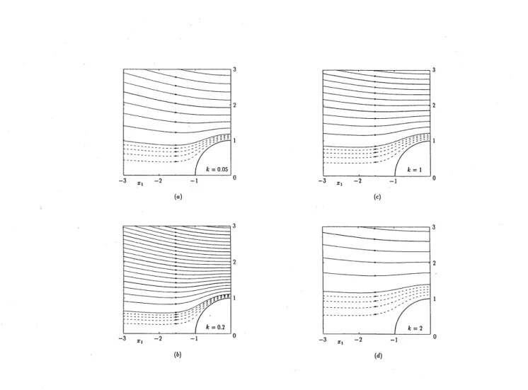
(ii) On the surface ofthe sphere, the velocity distribution function $\phi$ is discontinuous at $\zeta_{i}n_{i}=0$ because the nature of the velocity distribution function of the incoming molecules $(\zeta_{i}n_{i}<0)$ and that of the outgoing molecules $(\zeta_{i}n_{i}>0)$ are different. The discontinuity propagates into the gas along thecharacteristic of Eq. (1) ($i.e,$. in the direction of$\zeta_{i}$ for which $\zeta_{i}n_{i}=0$ onthe boundary). Therefore, at a given point $x_{i}$ in the gas, $\phi$ is discontinuous at $\zeta_{i}$ whose opposite vector $(-\zeta_{i})$ lies
onthecircularcone along which the edge of the sphere is viewed from $x_{i}$ $($Fig. $2)^{56}$. In the present
$(r, \zeta, \theta_{\zeta})$ space, the discontinuity of$\hat{\Phi}$
lies on the surface
$r\sin\theta_{\zeta}=1$, $(\pi/2\leq\theta_{\zeta}\leq\pi)$. (18) The position of the discontinuity is independent of the molecular speed $\zeta$. As the distance $r$
increases, the discontinuity decays owing to molecular collisions.
When we discretize the equations for $\hat{\Phi}$
, which include derivative terms $\partial\hat{\Phi}/\partial r$ and $\partial\hat{\Phi}/\partial\theta_{\zeta}$, we should not apply finite-difference approximations for differentiation to these terms across the discontinuity. Therefore, wedivide $(r, \zeta, \theta_{\zeta})$ spaceinto two regions by the discontinuity surface (18)
and apply standard finite-difference approximations in each region. In this scheme, the limiting values of $\hat{\Phi}_{\#}^{(n)}$ on the surface (18) from both sides are needed as the boundary condition. They are obtained separately by another finite-difference scheme along the characteristic (18). In the
region where the discontinuity has decayed sufficiently, we use astandard finite-difference scheme
for efficiency.
(iii) In the recursion formula to obtain $\hat{\Phi}_{\#}^{(n+1)}$, the collision integrals for $\hat{\Phi}[\mathcal{L}_{1}^{c}(\Phi_{c})-\mathcal{L}_{2}^{c}(\Phi_{C})$ and $\mathcal{L}_{1}^{s}(\hat{\Phi}_{s})-\mathcal{L}_{2}^{s}(\hat{\Phi}s)]$areevaluated by theuseof the dataat the preceding step $\hat{\Phi}_{\#}^{(n)}$. Since the collision
integrals take the majority of thecomputingtime ofthe whole analysis, their efficient computation is important. The computation of the collision integral$\mathcal{L}_{1}^{c}(\Phi_{C})-\mathcal{L}_{2}^{\mathrm{c}}(\Phi_{C})$ or$\mathcal{L}_{1}^{s}(\hat{\Phi}_{s})-\mathcal{L}^{s}2(\hat{\Phi}_{s})$ at the
lattice point of$(\zeta, \theta_{\zeta})$, say $(\zeta^{(i)}, \theta_{\zeta}^{(j)})$, is performed as
follows57.
The function$\hat{\Phi}$at the$n\mathrm{t}\mathrm{h}$ step is
expanded in terms of
a
set of basis functions $\mathrm{B}_{kl}(\zeta, \theta_{\zeta})$ as$\hat{\Phi}(r, \zeta, \theta_{\zeta})=\sum_{k,l}\hat{\Phi}(r, \zeta^{()}k, \theta_{\zeta}^{(})l)\mathrm{B}_{k}l(\zeta, \theta_{\zeta})$,
where the set of basis functions $\mathrm{B}_{kl}(\zeta, \theta_{\zeta})$ is chosen in such a way that
$\hat{\Phi}$
takes the exact value
$\hat{\Phi}(r, \zeta^{(k)}, \theta_{\zeta})(l)$ at everylattice point $(\zeta^{(k)}, \theta_{\zeta})(l)$ and is approximated by acontinuous and sectionally
quadratic function of$\zeta$and $\theta_{\zeta}$. Theset of the collision integrals of the basis functions forms alarge
matrix $\mathrm{M}_{(ij)}(k\iota)$ of (the number of the lattice $\mathrm{p}\mathrm{o}\mathrm{i}\mathrm{n}\mathrm{t}_{\mathrm{S}}$)$\cross$($\mathrm{t}\mathrm{h}\mathrm{e}$number of the lattice points) (about $4400\cross 4400$ in the present work), where both of the double indices $(ij)$ and $(kl)$ can be put in a
single index. Thus the collision integral $\mathcal{L}_{1}^{c}(\Phi_{\mathrm{C}})-\mathcal{L}_{2}^{C}(\Phi_{c})$ or $\mathcal{L}_{1}^{s}(\hat{\Phi}_{s})-\mathcal{L}^{s}2(\hat{\Phi}_{s})$ is expressed in the
product of the matrix $\mathrm{M}_{(ij)(l)}k$ and the column vector $\hat{\Phi}(r, \zeta^{(k)}, \theta_{\zeta})(l)$
as
$\sum_{k,l}\mathrm{M}_{(ij)}l$)
$r,,$
)$(k\hat{\Phi}(\zeta(k)\theta_{\zeta}(l)$ .
Sincethe twomatrices, corresponding to $\mathcal{L}_{12}^{c}-\mathcal{L}^{C}$ and $\mathcal{L}_{1}^{s}-\mathcal{L}^{s}2$
collision kernels), theycanbe computed beforehand and applied to other problems whose solutions
areexpressed by Eq. (7). Thus a veryefficient computation of the collision integralscanbecarried out. In the present computation, we usethe numerical collision kernels constructed in Ref. 12.
(iv) The problem is considered in a finite domain $(1 \leq r\leq r_{d}, 0\leq\zeta\leq\zeta_{d}, 0\leq\theta_{\zeta}\leq\pi)$ in $(r, \zeta, \theta_{\zeta})$ space, where $r_{d}$ and $\zeta_{d}$ are chosen properly depending on the situations. Because $\phi \mathrm{E}$
decays very rapidly as $\zetaarrow\infty$, the truncation of $\zeta$ at $\zeta=\zeta_{d}$ of a moderate value does not cause any problem. The solution $\phi$, however, approaches the value at infinity (12), say $\phi_{\infty}$, slowly as
$rarrow\infty(\sim r^{-m})$. Therefore, avery large$r_{d}$is required to obtain an accurate result if the condition
(12) is imposed directly at $r=r_{d}$. In order to avoid this difficulty, we match, at $r=r_{d}$, the
numerical solution with the asymptotic solution for large$r$. For$r>r_{\mathrm{A}}$ withlarge $r_{\mathrm{A}}$, the effective
length scale of variation of $\phi$ is $\mathrm{O}(r_{\mathrm{A}}\mathrm{L})$ [note that $\phi=\mathrm{O}(r^{-m})$] and thus the effective Knudsen
number$\ell_{0}/r_{\mathrm{A}}\mathrm{L}=\mathrm{K}\mathrm{n}/r_{\mathrm{A}}$ issmall. Therefore, the asymptotic theory of the Boltzmann equation for
small Knudsen$\mathrm{n}\mathrm{u}\mathrm{m}\mathrm{b}\mathrm{e}\mathrm{r}\mathrm{s}^{1}’ 2,4,5$can be
used to obtain the asymptotic solution for large$r$.
(v) For small Knudsen numbers, molecular collisions [or the collision term of Eq. (1)] play the dominant role in the behavior of the gas [or Eq. (1)]. Thus, a small error of computation of the collision integral of Eq. (1) is magnified in the solution. It is very inefficient (and unpractical in
thepresent situation) to carryoutmoredetailed computation than that carried out inRef. 12. We
can, however, bypass the difficulty by making use of the asymptotic $\mathrm{t}\mathrm{h}\mathrm{e}\mathrm{o}\mathrm{r}\mathrm{y}^{1,2,4,56,5}$ of the general
boundary-value problem of the Boltzmann equation for small Knudsen numbers. Let $\phi_{\mathrm{A}[\mathrm{N}]}$ be the
asymptotic solution of the problem:$\cdot$
$\phi=\phi_{\mathrm{A}1^{\mathrm{N}}}]+\mathrm{o}(k^{\mathrm{N}}+1)$
.
(19)The $\phi_{\mathrm{A}[\mathrm{N}]}$ is expressed by the
sum
ofthe global solution $\phi_{\mathrm{G}\mathrm{l}\mathrm{N}]}$ (hydrodynamic part) and its localcorrection $\phi_{\mathrm{K}[\mathrm{N}]}$ (Knudsen-layer and $\theta \mathrm{l}\mathrm{a}\mathrm{y}\mathrm{e}\mathrm{r}$ correction) near the sphere. Put $\psi$ as
$\phi=\phi_{\mathrm{G}1^{1]}}+\overline{\phi}$, (20)
then $\overline{\phi}$ is determined by
$\zeta_{i^{\frac{\partial\overline{\phi}}{\partial x_{i}}}}=\frac{1}{k}\mathcal{L}(\overline{\phi})-\zeta_{i}\frac{\partial(\phi_{\mathrm{G}[1]}-\phi_{\mathrm{G}}10])}{\partial x_{i}}$ , (21)
where the relation $\mathcal{L}(\phi_{\mathrm{G}}11])=k\zeta_{i}\partial\phi_{\mathrm{G}[}\mathrm{o}1/\partial X_{i}$ (see Refs. 1, 4, and 5) was used. Then, $\overline{\phi}=\mathrm{O}(k^{2})$
outside the Knudsen layer and $\overline{\phi}=\mathrm{O}(k)$ in the Knudsen layer since
$\phi_{\mathrm{G}[0}$] $=\phi_{\mathrm{A}1^{0}1}$ in thepresent
problem. Equation (21) is, theoretically, equivalent to Eq. (1), but is appropriate for numerical computation for small $k$, since the relative error of $\overline{\phi}$ obtained by Eq. (21) for rigorous or very
precise $\phi_{\mathrm{G}[11^{-\phi 0}}\mathrm{G}[]$ is of the sameorder of that of$\psi$ obtained by Eq. (1). V. Flow field and force on the sphere
A. Numerical solution
The numerical computation was, in most cases, carried out with the same lattice system that was used in Ref. 12. Some small improvements, as well as the method (v) in the previous section,
were
introducedwheresomedifficulty tomaintaintheaccuracyarises in thestraightforwardcomputation. The numericalsolutionsare supplementedby the analytical solutions for twoextreme
cases: small and infiniteKnudsen numbers in Sec. B.
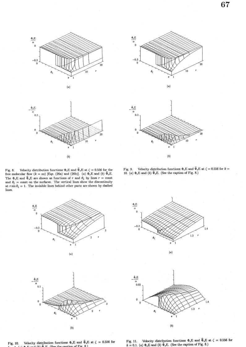
The macroscopic variables obtained from $\Phi_{c}$ and $\Phi_{s}$ by Eqs. $(17\mathrm{a})-(171)$ have simple $\theta$
depen-dence; that is, $\omega/\cos\theta,$ $\tau/\cos\theta,$ $u_{r}/\cos\theta,$ $u_{\theta}/\sin\theta$, etc. arefunctions of$r$ only. The distributioris
of$\omega/\alpha\cos\theta,$ $\tau/\alpha\cos\theta,$ $u_{r}/\alpha\cos\theta$, and $u_{\theta}/\alpha\sin\theta$
are
shown in Figs. $3(a)-4(b)$ forvarious $k$, wherethe free molecular solution and the Stokes solution without slip
are
also shown. The effect of the sphere with the nonuniformtemperatureonthe density and temperaturefields is larger and extendsin
a widerrangefor smaller Knudsen numbers. A flow is induced around asphere in the positive$x_{1}$ direction for $\alpha>0$, as a whole, irrespective of $k$. The flow vanishes at the two limiting cases
.
($k=0$ and $\infty$) [cf. Eqs. (27c), (30a), and $(30\mathrm{b})$], and reaches the maximum at $k=0.2\sim 0.4$. The
streamlines of the flow are shown for $k=0.05,0.2,1$ , and 2 in Figs. $5(a)-5(d)$, where the arrows
show the direction of the flow for $\alpha>0$. The flow speeds near the sphere (or maximum speeds)
for $k=0.05$ and 1 are fairly close, but the decay with the $\mathrm{d}\mathrm{i}\mathrm{s}\mathrm{t}\mathrm{a}\dot{\mathrm{n}}$ce from the sphere is faster for
$k=0.05$ [Figs.$4(a)$ and $4(b)$; compareFig. $5(a)$ with Fig. $5(c)$]. The flow velocity in the far field is
proportional to $1/r$ commonly to $k$; the constant of proportion, however, depends on $k$. The heat
flow $\mathrm{Q}_{r}/\alpha\cos\theta$ at $r=1$, which is important to derive the drag and thermal force of a spherical
particle with an arbitrary thermal conductivity, is shown in Fig. 6. Itvanishes at $k=0$ [Eq. (31)], increases monotonically as $k$ increases, and reaches $1/\sqrt{\pi}$ at $k=\infty$ [Eq. $(28\mathrm{b})$].
The force $\mathrm{F}_{i}$ acting on the sphere is expressed as
$\mathrm{F}_{1}$ $=$ $p_{0}\mathrm{L}^{2}\alpha h(k)$, (22a)
F2
$=$ $\mathrm{F}_{3}=0$, (22b)where$h$ is given in Fig. 7and Table I. The$h$ is zero at$k=0$ [Eq. (32)], decreases monotonicallyas $k$ increases, and $\mathrm{r}\mathrm{e}\mathrm{a}\mathrm{c}\mathrm{h}\mathrm{e}\mathrm{S}-\pi/3$ at $k=\infty$ [Eq. (29)]. Thus, the force is in the negative
$x_{1}$ direction
for $\alpha>0$; that is, the force is in the opposite direction to that of the overall flow. It is noted that
the sphere is subject to a force at $k=\infty$ although there is no flow. This is a typical feature of a
free molecular$\mathrm{g}\mathrm{a}\mathrm{s}58-60,5$. (In the continuum gas or the Navier-Stokes gaswithout extemal forces,
no flow corresponds to no forceon a closed body.)
In the free molecular flow, the velocity distribution function of the molecules impinging on a
small surface element $d\mathrm{S}$ on the sphere is the corresponding part of the distribution at infinity.
The mass flux and the magnitude of the momentum flux due to the molecules impinging on $d\mathrm{S}$,
therefore, are uniform over the sphere; the direction of the momentum flux is normal to $d\mathrm{S}$. Thus,
the total momentum flux to the sphere due to the impinging molecules vanishes. The mass flux dueto the molecules outgoing from $d\mathrm{S}$ is also uniformoverthe sphere, since there is noevaporation or condensation on the sphere. Onthe other hand, the molecules outgoing from the hotter side of the sphere havehigher speedontheaverage; correspondingly the magnitude of the momentum flux
due to the outgoing molecules is larger on the hotter side, because of the uniform mass flux. The totalmomentum flux leaving the sphere, therefore, is in the directionto the hotter from the colder side of the sphere. Thus, the net momentum flux to the sphere of all the molecules (impinging and outgoing) and, therefore, the force on the sphere arein the direction to the colder from the hotter side of thesphere, $i.e.$, inthenegative$x_{1}$ direction for$\alpha>0$. (Inthissituationthemass flux
vanisheseverywhere in thegas aswellas onthe sphere,although this isnotintuitively$\mathrm{o}\mathrm{b}_{\mathrm{V}}\mathrm{i}\mathrm{o}\mathrm{u}\mathrm{S}58,59.$)
Molecular collisions transfer the momentum flux of the outgoing molecules from the sphere, which is totally inthe$x_{1}$ directionfor$\alpha>0$andescapesto infinity in the free molecular case, to surrounding
gas molecules. Thus, a flow is induced, and the force on the sphere is decreased.
Thecauseofthe flowcanbe understood locally asfollows. Considerthemomentum transferred
to $d\mathrm{S}$ from thegas. Here the component of the momentum tangential (or parallel) to $d\mathrm{S}$ is ofour
interest. Then we only have to estimate the momentum flux due to the molecules impinging on
$d\mathrm{S}$, since themomentum flux due to the molecules outgoingfrom $d\mathrm{S}$ has
no
tangential componentin the case of the diffuse reflection. In the free molecular gas, the momentum flux due to the
impinging molecules, which is not affected by the sphere, does not haveany tangential component.
Forfinite Knudsen numbers, the velocity distribution around the sphere, of the molecules directing toward the sphere is also affected by the sphere. The molecules impinging on $d\mathrm{S}$ come directly
(or without collision with other molecules) from a region about a mean free path away from $d\mathrm{S}$.
Thus, the molecules impinging on $d\mathrm{S}$ from the hotter (colder) side have higher (lower) speed on
component toward the colder side. Thus, the surface element $d\mathrm{S}$ is subject to a force toward the
colder side along $d\mathrm{S}$. Thegas is subject to its reaction, and asteady flow is induced in sucha way
that themomentum flux duetothe flow inducedcounterbalancesthe original momentumflux (the thermal creep $\mathrm{e}\mathrm{f}\mathrm{f}\mathrm{e}\mathrm{c}\mathrm{t}6-8$). The flow speed increases as the Knudsen number decreases, since more
impinging molecules areaccelerated or decelerated bymolecularcollisions. If the Knudsen number becomes very small, however, the molecules proceed only a very short distance before the next collision, and the velocity distribution function becomes isotropic. Thus thetangential momentum flux vanishes and no flow is induced in the continuum limit. The flow, therefore, has its maximum
at some intermediate Knudsen number.
The force on the spherecan be computed by integrating the momentum flux
over
any control surface enclosing the sphere. In principle thisserves
a good accuracy test of computation, but in practice it is toosevere atest to be applied toalarge controlsurface, where the force is obtained asa small quantity integrated over alarge area. Small
errors
in local variables are multiplied by the factor$r_{c}^{2}$, where$r_{c}$is the characteristic dimension of the control surface, and lead to aconsiderable
error
in the force. The data in Table I are computed on the sphere. For a test of the accuracy ofthe computation, the variation (max–min) of$h$ computed on the control spheres $r=r^{(i)}$ for all the lattice points $r^{(i)}$ between $r=1$ and 4 is also shown in Table I.
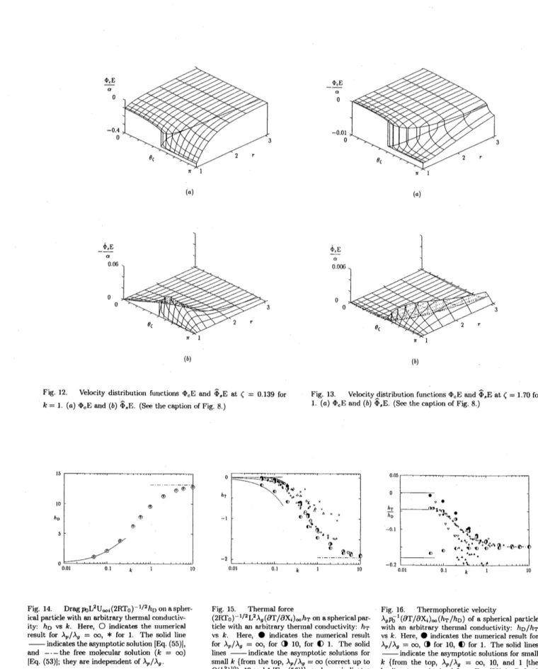
The $\Phi_{c}$ and $\Phi_{s}$ at $\zeta=$ 0.556 over $r\theta_{\zeta}$ plane are shown in Figs. $8(a)-11(b)$. The surfaces
$\Phi_{c}$
and $\Phi_{s}$ are separated by their discontinuities at $r\sin\theta_{\zeta}=1(\pi/2\leq\theta_{\zeta}\leq\pi)$ [cf. Sec. IV(ii)].
Thediscontinuity is the border of the region $[\pi-\mathrm{A}\mathrm{r}\mathrm{C}\sin(1/r)\leq\theta_{\zeta}\leq\pi]$, say region I, that can be
reached directly bya moleculefrom the sphere. In the free molecular flow$(k=\infty)$,whose analytical
solution is given in Sec. $\mathrm{B}$, the velocity distribution function $\phi$ is constant along a characteristic
of Eq. (1) and it is equal to the value at the starting point of the characteristic (the sphere or infinity). Thus $\phi$ (and therefore $\Phi_{c}$ and $\Phi_{s}$) is zero in the region $[0\leq\theta_{\zeta}<\pi-\mathrm{A}\mathrm{r}\mathrm{c}\sin(1/r)]$, say
region II. The size of the discontinuity of $\phi$ is invariant along the discontinuity $(r\sin\theta_{\zeta}=1)$, but
that of$\Phi_{c}$ or $\Phi_{s}$ should be noted to vary along $r\sin\theta_{\zeta}=1$ [Figs. $8(a)$ and $8(b)$]. For a finite value
of$k,$ $\phi$ondifferent characteristics interacts bymolecularcollisions, and $\Phi_{c}$ and
$\Phi_{s}$ deviate from the
free molecular ones in Figs. $8(a)$ and $8(b)$. At $k=10,$ $\Phi_{c}$ and $\Phi_{s}$ are little affected by molecular
collisions in region II, but they are affected considerably some distance away from the sphere in region I [Figs. $9(a)$ and $9(b)$]. The discontinuity decays in several mean free paths $(r=20\sim 30)$
from the sphere. At $k=1$, the effect of molecular collisions is appreciable over all $r$ in region I and within some distance from the sphere in region II [Figs. $10(a)$ and $10(b)$]. It is stronger near
thediscontinuity. Thediscontinuity also decays in several mean free paths $(r=2\sim 3)$ from the
sphere. The overall feature is similar to that of the case $k=10$. At $k=0.1$, the overall feature is considerably different; the effect of collision prevails over the whole region [Figs. 11$(a)$ and 11$(b)$].
The discontinuity decays in a much shorter distance than the
mean
free path. As explained inRef. 56, thediscontinuity decays in several (mean) free paths along the characteristic $r\sin\theta_{\zeta}=1$, butthe distance from the sphere to the part of the characteristic wherediscontinuityis appreciable is much smaller than the mean free path, because the characteristic is still nearly parallel to the surface of the sphere for several meanfree paths in thecaseofsmall Knudsen numbers (cf. Fig. 7in
Ref. 56). Afterthediscontinuitydisappears, $\Phi_{c}$and $\Phi_{s}$ arefurtherdeformedand becomesmoother
in a few
mean
free paths $(r=1.2\sim 1.3)$ from the sphere. Fhrther away from the sphere their deformation is roughlyexpressed with a global scale change (similar deformation) and theyvanish at infinity. The region withdiscontinuityis the$S1\mathrm{a}\mathrm{y}\mathrm{e}\mathrm{r}^{61}’ 56$ at the bottom of theKnudsenlayer, theintermediate region is the Knudsen layer, and the outer region is the hydrodynamic $\mathrm{r}\mathrm{e}\mathrm{g}\mathrm{i}\mathrm{o}\mathrm{n}^{1}’ 2,4,5$.
Figures $8(a)-11(b)$ show $\Phi_{c}$ and $\Phi_{s}$ for a representative molecular speed $(\zeta=0.556)$. For smaller
(or larger) molecularspeed, the free path of the moleculeis smaller (or larger), and therefore the behavior of$\Phi_{c}$ and $\Phi_{s}$ shows the feature of smaller (or larger) Knudsen number. The surfaces
$\Phi_{c}$
and $\Phi_{s}$ for $k=1$ at $\zeta=0.139$ and those for $k=1$ at $\zeta=1.70$
are
shown in Figs. $12(a)-13(b)$.or BGK) $\mathrm{e}\mathrm{q}\mathrm{u}\mathrm{a}\mathrm{t}\mathrm{i}\mathrm{o}\mathrm{n}62-64$ by the same finitedifference method. Some
of the results are shown in Figs. 6and 7forcomparison. Theway of comparing the results of different molecular models is not unique. The present problem contains two parameters $\alpha$ and $k$. The parameter $k$ can be replaced
by $\mu_{g}/p_{0}\mathrm{L}(\mathrm{R}\mathrm{T}\mathrm{o})1/2,$ $\lambda_{g}(\mathrm{R}\mathrm{T}\mathrm{o})1/2/m\mathrm{L}\mathrm{R}$, or $(\mu_{\mathit{9}}\lambda_{g})^{1/}2\mathrm{T}12/\mathrm{o}^{/}p0\mathrm{L}$, where
$\mu_{g}$ and $\lambda_{g}$ are, respectively,
the viscosity and thermal conductivity of thegasat the reference state, since $\mu_{g}$ and $\lambda_{g}$ arerelated
to$\ell_{0}$ as$\mu_{g}=(\sqrt{\pi}/2)\gamma_{1}p\mathrm{o}(2\mathrm{R}\mathrm{T}\mathrm{o})-1/2\ell_{0}$ and $\lambda_{g}=(5/4)\sqrt{\pi}\gamma_{2}p0(2\mathrm{R}\mathrm{T}\mathrm{o})-1/2\mathrm{R}\ell_{0}$, where$\gamma_{1}=1.270042$
and $\gamma_{2}=$ 1.922284 for the hard-sphere molecular gas, and $\gamma_{1}=\gamma_{2}=1$ for the BKW model.4,10
The result of comparison, however, depends on the choice of the parameter, because the relation between $\ell_{0}$ and
$\mu_{g},$ $\lambda_{g}$, or $(\mu_{g}\lambda_{g})^{1/}2$ differs by molecular models. When $\mu_{g}/p_{0}\mathrm{L}(\mathrm{R}\mathrm{T}\mathrm{o})1/2$ (or $\mu_{g}$)
is taken as the basic parameter instead of $k$ (or $\ell_{0}$), $k$ for the BKW model is related to $k$ for the hard-sphere moleculargas as
$k$ (BKW) $=1.270042k$ (hard sphere). (23)
With$\lambda_{g}(\mathrm{R}\mathrm{T}0)1/2/p_{0}\mathrm{L}\mathrm{R}$ (or $\lambda_{\mathit{9}}$) as the basic parameter,
$k$ (BKW) $=1.922284k$ (hard sphere). (24)
With $(\mu_{g}\lambda_{g})1/2\mathrm{T}/0/120p\mathrm{L}$ [or $(\mu_{g}\lambda_{g})^{1/}2$] as the basic parameter,
$k$ (BKW) $=1.562492k$ (hard sphere). (25)
In Fig. 6 (7) the conversion (25) [(24)] is used to show the BKW result.
The computation was carried out on HP 9000730 computers at our laboratory (for the BKW
equation) and FUJITSU VP-2600 computer at the Data Processing Center of Kyoto University (for the Boltzmann equation for hard-sphere molecules).
B. Free molecular solution and asymptotic solution for small Knudsen numbers
Here, wesummarize the analytical solutions for two extremecases: the free molecular solution and the asymptotic solution for small Knudsen numbers. The free molecular solution canbe easily obtained as follows:
$\frac{\Phi_{c}}{\alpha}$
$=$ $\{$
$0$, $[0\leq\theta_{\zeta}<\pi-\mathrm{A}\mathrm{r}\mathrm{c}\sin(1/r)]$, $(\zeta^{2}-2)[r\sin\theta 2\zeta-\cos\theta\zeta(1 -r^{2}\sin^{2}\theta\zeta)^{1/2}]$,
$[\pi-\mathrm{A}\mathrm{r}\mathrm{C}\sin(1/r)\leq\theta_{\zeta}\leq\pi]$, (26a) $\frac{\Phi_{s}}{\alpha}$ $=$ $\{$ $0$, $[0\leq\theta_{\zeta}<\pi-\mathrm{A}\mathrm{r}\mathrm{c}\sin(1/r)]$, $-\zeta^{-1}(\zeta^{2}-2)[r\cos\theta_{\zeta}+(1 -r^{2}\sin^{2}\theta\zeta)^{1/2}]$, $[\pi-\mathrm{A}\mathrm{r}\mathrm{C}\sin(1/r)\leq\theta_{\zeta}\leq\pi]$, (26b)
$\frac{\omega}{\alpha\cos\theta}$ $=$ $- \frac{1}{12}[2r-(2+r^{-2-2})(1-r)^{1/2}r+r^{-2}]$, (27a)
$\frac{\tau}{\alpha\cos\theta}$ $=$ $\frac{1}{6}[2r-(2+r^{-2-2})(1-r)^{1/2}r+r^{-2}]$, (27b)
$\frac{u_{r}}{\alpha\cos\theta}$ $=$ $\frac{u_{\theta}}{\alpha\sin\theta}=0$, (27c)
especially, at $r=1$
$\frac{\mathrm{Q}_{r}}{\alpha\cos\theta}=\frac{1}{\sqrt{\pi}}$, (28b)
$h=- \frac{\pi}{3}$
.
(29)No flow is induced in the free molecular case, which is proved under a more general condition in Refs. 58 and 59. Various examples of forces on heated bodies in a freemolecular gas at rest are
given in Refs. 60, 65, and 5.
The asymptotic solution for small Knudsen numberscanalso be easily obtained with the aid of the asymptotic$\mathrm{t}\mathrm{h}\mathrm{e}\mathrm{o}\mathrm{r}\mathrm{y}^{1,2,4,56,5}$ ofthe boundary value problem of the Boltzmann equationasfollows:
$\frac{u_{r}}{\alpha\cos\theta}$ $=$ $\mathrm{K}_{1}k(-r^{-1}+r^{-3})$, (30a)
$\frac{u_{\theta}}{\alpha\sin\theta}$ $=$ $\frac{1}{2}\mathrm{K}_{1}k(r^{-1}+r^{-3})+\frac{1}{2}k\mathrm{Y}_{1}(\eta)$, (30b)
$\frac{\omega}{\alpha\cos\theta}$ $=$ $-(1-2d_{1}k)r^{-2}-2k\Omega 1(\eta)$, $(30_{\mathrm{C}})$
$\frac{\tau}{\alpha\cos\theta}$ $=$ $(1-2d_{1}k)r^{-}-22k\Theta_{1}(\eta)$, (30d)
$\frac{\mathrm{Q}_{r}}{\alpha\cos\theta}=\frac{5}{2}\gamma_{2}(1-2d1k)kr^{-3}-2k^{2}\int_{\eta}^{\infty}\mathrm{H}_{\mathrm{B}}(y)dy$, (31)
$h=4\pi\gamma_{1}\mathrm{K}1k^{2}$, (32)
where $d_{1}$ and $\mathrm{K}_{1}$ are, respectively, thetemperaturejump and thermal creep slip coefficients $\{d_{1}=$
2.4001, $\mathrm{K}_{1}=-0.6463$ (hard sphere); $d_{1}=$ 1.30272, $\mathrm{K}_{1}=$
-0.38316
(BKW) (Refs.8
and 57) $[d_{1}$(here) $=\beta$ (Ref. 57) and $\mathrm{K}_{1}$ (here) $=-\beta_{\mathrm{B}}$ (Ref. 8)$]\}$; $\Theta_{1}(\eta),$ $\Omega_{1}(\eta),$ $\mathrm{Y}_{1(\eta})$, and $\mathrm{H}_{\mathrm{B}}(\eta)$, called the
Knudsen-layer functions, are functions of the stretched coordinate $\eta$ defined $\eta=(r-1)/k$ and
tabulated in Refs. 8 and 57
{
$[\Theta_{1}(\eta), \Omega_{1}(\eta), \mathrm{H}_{\mathrm{B}}(\eta), \eta]$ (here, Ref. $4$) $=[\Theta(x_{1}), \Omega(x_{1}), \mathrm{H}\mathrm{B}(X_{1}), x_{1}]$ (Ref. 8) and $[\mathrm{Y}_{1}(\acute{\eta}),\dot{\eta}]$(here, Ref. $4$) $=[-2\mathrm{C}(X_{1}), x_{1}]$ (Ref. 57)$\}$. Equations $(30\mathrm{a})-(3\mathrm{o}\mathrm{d})$ arecorrectup to the order of$k$, and Eqs. (31) and (32) up to the order of$k^{2}$.
VI. Drag and thermal force problems of a spherical particle with an arbitrary ther-mal conductivity
In this section the drag and thermal force problems ofa spherical particle with an arbitrary thermal conductivity are considered. The drag problem (Problem D) is concerned with a particle placed in a uniform flow [velocity: $\mathrm{U}_{\infty i}=((2\mathrm{R}\mathrm{T}0)^{1/}2)u\mathrm{o}\infty$
”$0$ , pressure: $p_{0}$, temperature: $\mathrm{T}_{0}$] of a gas, and the thermal force problem (Problem T) is concemed with a particle placed in a gas
at rest with a small uniform temperature gradient [pressure: $p_{0}$, temperature: $\mathrm{T}=\mathrm{T}_{0}(1+\beta x_{1})$,
temperaturegradient: $(\mathfrak{M}/\partial \mathrm{X}_{i})_{\infty}=(\beta \mathrm{T}/\mathrm{L}, 0,0)]$. These problems for a spherical particle with a
uniform surface temperature (or a spherical particle with a very large thermal conductivity) are
studied in Refs. 12 and 47. We will show that the solution of Problem $\mathrm{D}$ or $\mathrm{T}$ for the general
case (arbitrary thermal conductivity) can be constructed with that of Problem $\mathrm{D}$ or $\mathrm{T}$ for the
specialcase (infinite thermal conductivity) and that of the problem studied in Secs. III-V. In the following analysis thesamenondimensional variablesasthose introduced inSec.II areusedwith the additional subscript $\mathrm{D}$ or$\mathrm{T}$ to indicate Problem$\mathrm{D}$ orT. The only exception is the nondimensional
force$h$ on the particle for which $h,$ $h_{\mathrm{D}}$, and $h_{\mathrm{T}}$ are nondimensionalized bydifferent quantities, $i.e.$,
by$p_{0}\mathrm{L}^{2}\alpha,$ $p_{0}\mathrm{L}2\mathrm{U}\infty i(2\mathrm{R}\mathrm{T}0)-1/2$, and $\mathrm{L}^{2}\lambda_{g}(\partial \mathrm{T}/\partial \mathrm{X}_{i})_{\infty}(2\mathrm{R}\mathrm{T}_{0})^{-1}/2$ , respectively.
In the problems for a particle with a finite value of the thermal conductivity, the fiow field of
to be analyzed simultaneously. The problems aregiven by the following systems. The behavior of thegas is described by Eq. (1):
$\zeta_{i^{\frac{\partial\phi_{\mathrm{D}\mathrm{T}}}{\partial x_{i}}}}=\frac{1}{k}\mathcal{L}(\phi_{\mathrm{D}\mathrm{T}})$, ($\mathrm{D}\mathrm{T}=\mathrm{D}$ or T).
Thetemperature $\tau_{p}$ inside the particle is governed by the Laplace equation:
$\frac{\partial^{2}\tau_{p}}{\partial x_{i}^{2}}=0$. (33)
On the surface$\mathrm{S}$ ofthe particle, in addition to the diffuse reflection condition:
$\phi_{\mathrm{D}\mathrm{T}}(X_{i}\in \mathrm{S}, \zeta i)=(\zeta 2-2)\tau_{p}|\mathrm{s}-2\pi 1/2\int_{\zeta_{i}}n_{i}<01\zeta_{j}nj\psi_{\mathrm{D}\mathrm{T}}\mathrm{E}d\zeta d\zeta_{2}d\zeta_{3}$, $(\zeta_{i}n_{i}>0)$, (34)
thecondition of continuity of the energy flux through the surface $\mathrm{S}$ is required:
$\frac{\partial\tau_{p}}{\partial x_{i}}|_{\mathrm{S}}n_{i}=-\frac{4}{5}k^{-}1-1\frac{\lambda_{g}}{\lambda_{p}}\gamma_{2}\mathrm{Q}i\mathrm{D}\mathrm{T}|\mathrm{S}n_{i}$ , (35)
where $\lambda_{p}$ is the thermal conductivity of the particle. The condition at infinity, which is thesame as that in Ref. 12 or 47, is given
$\phi_{\mathrm{D}\mathrm{T}}arrow\phi_{\mathrm{D}\mathrm{T}\infty}$, (36)
where
$\psi_{\mathrm{D}\infty}$ $=$ $2\zeta_{1}u_{\infty}$, (37)
$\phi_{\mathrm{T}\infty}$ $=$ $\beta[(\zeta^{2}-\frac{5}{2})_{X_{1}}-k\zeta_{1}\mathrm{A}(\zeta)]$, (38)
where$\mathrm{A}(\zeta)$ is the solution of thefollowingintegral $\mathrm{e}\mathrm{q}\mathrm{u}\mathrm{a}\mathrm{t}\mathrm{i}\mathrm{o}\mathrm{n}:66,10$
$\{$ $\mathcal{L}[\zeta_{i}\mathrm{A}(\zeta)]=-\zeta_{i(}\zeta^{2}-\frac{5}{2})$, subsidiary condition: $\int_{0}^{\infty}\zeta^{4}\mathrm{A}(\zeta)\exp(-\zeta^{2})d\zeta=0$. (39) We put
$\phi_{\mathrm{D}\mathrm{T}}=\phi \mathrm{I}+\phi \mathrm{D}\mathrm{T}(\lambda_{\mathrm{P}}=\infty)$, (40)
where $\phi_{\mathrm{D}\mathrm{T}}(\lambda_{p}=\infty)$ is the solution $\phi_{\mathrm{D}\mathrm{T}}$ for the particle with a uniform temperature or $\lambda_{\mathrm{p}}=\infty$.
The first term $\phi_{\mathrm{I}}$ on the right hand side in Eq. (40), dependent on $\mathrm{D}$ or $\mathrm{T}$, is denoted by $\phi_{\mathrm{I}(\mathrm{D}\mathrm{T}}$
) when discrimination is required. Then, $\phi_{\mathrm{I}}$ satisfies thesame equation as $\phi_{\mathrm{D}\mathrm{T}}$ or Eq. (1):
$\zeta_{i^{\frac{\partial\phi_{\mathrm{I}}}{\partial x_{i}}=}}\frac{1}{k}\mathcal{L}(\phi \mathrm{I})$
.
(41)The diffuse reflection condition (34) is reducedto
$\phi_{\mathrm{I}}(x_{i}\in \mathrm{s}, \zeta_{i})=(\zeta^{2}-2)_{\mathcal{T}}p|_{\mathrm{s}}-2\pi 1/2\int_{\zeta_{i}n_{i}<}0\zeta jn_{j}\phi \mathrm{I}\mathrm{E}d\zeta 1d\zeta 2d\zeta 3$, $(\zeta_{i}n_{i}>0)$, (42)
and the conditionofcontinuity of the
energy
flux (35) isThecondition at infinity is simply
$\phi_{\mathrm{I}}arrow 0$
.
(44)The problems become simple for a spherical particle. Noting that $\tau_{\mathrm{p}}=\alpha_{\mathrm{I}}r\cos\theta[\alpha_{1}$ is also
denoted by $\alpha_{\mathrm{I}(\mathrm{D}\mathrm{T})}$ for discrimination] is a solution of Eq. (33), we find that
$\phi_{\mathrm{I}}$ in the form of
Eq. (7), $i.e_{f}$
.
$\phi_{\mathrm{I}}=\Phi c\mathrm{I}(r, \zeta, \theta\zeta)\cos\theta+\zeta\theta\Phi s\mathrm{I}(r, \zeta, \theta\zeta)\sin\theta$, (45)
is consistent with the boundary conditions as well as Eq. (41). That is, $\Phi_{c\mathrm{I}}$ and $\Phi_{s\mathrm{I}}$ are governed
by Eqs. (9) and (10) (with $\Phi_{C}=\Phi_{c\mathrm{I}}$ and $\Phi_{S}=\Phi_{s\mathrm{I}}$). Corresponding to Eqs. (42) and (43),
$\{$
$\Phi_{c\mathrm{I}}=(\zeta^{2}-2)\alpha_{\mathrm{I}}+2\pi^{3/2}\int_{0}^{\infty}\int_{0}^{\pi/2}\zeta 3\mathrm{i}\mathrm{n}2\theta\zeta\Phi c\mathrm{I}\mathrm{E}d\mathrm{s}\theta\zeta d\zeta$,
$\Phi_{s\mathrm{I}}=0$,
$(\pi/2\leq\theta_{\zeta}\leq\pi)$, (46)
and
$\mathrm{Q}_{r1}|_{r}=1=-\mathrm{Q}r\mathrm{D}\mathrm{T}(\lambda=p\infty)|r=1-\frac{5}{4}k\gamma 2\frac{\lambda_{p}}{\lambda_{g}}\alpha \mathrm{I}\cos\theta$. (47)
From Eq. (44), the condition at infinity is
$\Phi_{c\mathrm{I}}arrow 0$, $\Phi_{s\mathrm{I}}arrow 0$
.
(48)The solution of Eqs. (9) and (10), with $\Phi_{c}=\Phi_{c\mathrm{I}}$ and $\Phi_{s}=\Phi_{s\mathrm{I}}$, under the boundary conditions
(46) and (48), with undetermined $\alpha_{\mathrm{I}}$, is given in terms of
$\Phi_{c}$ and $\Phi_{s}$ in Secs. III-Vas
$( \Phi_{c\mathrm{I}}, \Phi_{s\mathrm{I}})=\frac{\alpha_{\mathrm{I}}}{\alpha}(\Phi_{c}, \Phi S)$, (49)
[cf. Eqs. (11) and (12)]. In other words the solution is obtained by replacing $\alpha$ in the solution in Secs. III-V by $\alpha_{\mathrm{I}}$. Thus$\mathrm{Q}_{r\mathrm{I}}$ isgiven by $(\alpha_{\mathrm{I}}/\alpha)\mathrm{Q}_{r}$with $\mathrm{Q}_{r}$ inSecs. III-V. Substituting this $\mathrm{Q}_{r\mathrm{I}}|_{r=1}$
in Eq. (47), weobtain the constant $\alpha_{\mathrm{I}}$ as
$\alpha_{1}=\frac{-(4/5)k-1-\gamma_{2}(1\lambda g/\lambda_{p})[\mathrm{Q}_{r}\mathrm{D}\mathrm{T}(\lambda_{\mathrm{p}}=\infty)/\cos\theta]}{1+(4/5)k-1\gamma_{2}^{-1}(\lambda_{g}/\lambda \mathrm{p})(\mathrm{Q}r/\alpha\cos\theta)}|_{r=1}$, (50)
It is noted here that $\mathrm{Q}_{r\mathrm{D}}(\lambda_{p}=\infty)/u_{\infty}\cos\theta,$ $\mathrm{Q}_{r\mathrm{T}}(\lambda_{\mathrm{p}}=\infty)/\beta\cos\theta$, and $\mathrm{Q}_{r}/\alpha\cos\theta$ at $r=1$ are
functions of$k$ only.
Thus, the solution of the dragorthermal force problem foraspherical particle withanarbitrary thermal conductivity is given by thesum [Eq. (40)] of the corresponding solution for the particle with $\lambda_{p}=\infty$ and the solution inSecs. III-V with $\alpha=\alpha_{\mathrm{I}}$. Thereforethe drag$\mathrm{F}_{\mathrm{D}i}$ and the thermal
force$\mathrm{F}_{\mathrm{T}i}$ aregiven by
$\mathrm{F}_{\mathrm{D}i}$ $=$
$P\mathrm{o}^{\mathrm{L}^{2}}\mathrm{U}_{\infty i(}2\mathrm{R}\mathrm{T}0)-1/2h_{\mathrm{D}}$, (51a)
$h_{\mathrm{D}}$ $=$ $h_{\mathrm{D}}( \lambda_{p}=\infty)+\frac{\alpha_{\mathrm{I}(\mathrm{D})}}{u_{\infty}}h$, (51b)
with
$\frac{\alpha_{\mathrm{I}(\mathrm{D})}}{u_{\infty}}=\frac{-(4/5)k-1-\gamma_{2}(1\lambda_{g}/\lambda)p[\mathrm{Q}_{r}\mathrm{D}(\lambda_{p}=\infty)/u_{\infty}\cos\theta]}{1+(4/5)k-1\gamma_{2}^{-}1(\lambda_{g}/\lambda)p(\mathrm{Q}_{r}/\alpha\cos\theta)}|_{r=1}$, (51c)
and
$\mathrm{F}_{\mathrm{T}i}$ $=$ $(2 \mathrm{R}\mathrm{T}\mathrm{o})-1/2\mathrm{L}2\lambda g(\frac{\partial \mathrm{T}}{\partial \mathrm{X}_{i}})_{\infty}h_{\mathrm{T}}$, (52a) $h_{\mathrm{T}}$ $=$ $h_{\mathrm{T}}( \lambda_{\mathrm{P}}=\infty)+\frac{4}{5}k-1\gamma 2-1_{\frac{\alpha_{\mathrm{I}(\mathrm{T})}}{\beta}h}$, (52b)
with
$\frac{\alpha_{\mathrm{I}(\mathrm{T})}}{\beta}=\frac{-(\lambda_{g}/\lambda)p[\mathrm{Q},\mathrm{r}(\lambda=\infty)p/(5/4)k\gamma 2\beta\cos\theta]}{1+(4/5)k-1\gamma_{2}^{-}1(\lambda_{g}/\lambda)p(\mathrm{Q}r/\alpha\cos\theta)}|_{r=1}$ (52c)
Here, $h_{\mathrm{D}}$ and $h_{\mathrm{T}}$ are functions of$k$ and $\lambda_{p}/\lambda_{g}$; the flow velocity $\mathrm{U}_{\infty i}$ in Eq. (51a) and the
tem-perature gradient $(\mathfrak{M}/\partial \mathrm{X}_{i})_{\infty}$ in Eq. (52a) do not have to be in the
$\mathrm{X}_{1}$ direction. The necessary
information to obtain $h_{\mathrm{D}}$ and $h_{\mathrm{T}},$ $i.e_{\text{ノ}}.h_{\mathrm{D}}(\lambda_{p}=\infty),$ $h_{\mathrm{T}}(\lambda_{p}=\infty),$ $\mathrm{Q}_{r\mathrm{D}}(\lambda_{p}=\infty)|_{r=1}/u_{\infty}\cos\theta$, $\mathrm{Q}_{r\mathrm{T}}(\lambda_{p}=\infty)|_{r=1}/(5/4)k\gamma_{2}\beta\cos\theta,$ $h$, and $\mathrm{Q}_{r}|_{r=1}/\alpha\cos\theta$, is given in Table II. (The
nondimen-sional forces $h_{\mathrm{D}}(\lambda_{p}=\infty)$ and $h_{\mathrm{T}}(\lambda_{p}=\infty)$ are, respectively, denoted by $h_{\mathrm{D}}$ in Ref. 12 and $h_{\mathrm{T}}$ in
Ref. 47. The third and fourth quantities, related to Refs. 12 and 47 as well as the first and second,
are not shown in these papers.) The asymptotic form of$h_{\mathrm{D}}$ and $h_{\mathrm{T}}$ for large and small $k$ are as follows: Theleading terms of$h_{\mathrm{D}}$ and $h_{\mathrm{T}}$ for large $k$ are
$h_{\mathrm{D}}$ $=$ $h_{\mathrm{D}}( \lambda_{p}=\infty)=\frac{2}{3}\sqrt{\pi}(\pi+8)$, (53)
$h_{\mathrm{T}}$ $=$ $h_{\mathrm{T}}( \lambda_{p}=\infty)=-\frac{32\sqrt{\pi}}{15}\gamma_{2}^{-}1\int_{0}^{\infty}\zeta^{52}\mathrm{A}(\zeta)\exp(-\zeta)d\zeta$, (54)
which are independent of$\lambda_{p}/\lambda_{g}$. The $h_{\mathrm{D}}$, up to $\mathrm{O}(k^{2})$, and $h_{\mathrm{T}}$, up to $\mathrm{O}(k)$, for small $k$ are
$h_{\mathrm{D}}$ $=$ $h_{\mathrm{D}}(\lambda_{p}=\infty)=6\pi\gamma_{1}k(1+k0^{k})$, (55)
$h_{\mathrm{T}}$ $=$ $\frac{16\pi}{5}\frac{3\lambda_{g}/\lambda_{p}}{1+2\lambda_{\mathit{9}}/\lambda_{p}}\gamma 1\gamma_{2^{-}1}\mathrm{K}k1$, (56)
where $k_{0}$ is the shear slip coefficient [$k_{0}=-1.2540$ (hard sphere), $=$
-1.01619
(BKW);$k_{0}$ (here)
$=-\beta_{\mathrm{A}}$ (Ref. 8)$]$. Thedrag $h_{\mathrm{D}}$ is independent of$\lambda_{p}/\lambda_{g}$ up to the order of$k^{2}$.
The profile$h_{\mathrm{D}}$ vs$k$ and $h_{\mathrm{T}}$ vs $k$ areshown for several $\lambda_{p}/\lambda_{g}$ in Figs. 14 and 15 respectively. In
these figures, the asymptotic solutions for large and small $k$ are also shown. Experimental results of the thermal force by several authors, which range from $k\cong$ 0.047 to 3.2, are also shown in Fig. 15. The numerical and experimental results, except the data in Ref. 32, agreewell, especially for small Knudsen numbers. The drag$h_{\mathrm{D}}$depends littleon$\lambda_{p}/\lambda_{g}$, but the thermal force$h_{\mathrm{T}}$depends
considerably on $\lambda_{p}/\lambda_{g}$. The numerical and experimental results, which are limited to $k\sim>0.05$,
do not show negative thermophoresis (Fig. 15). The asymptotic solution for very large $\lambda_{p}/\lambda_{g}$ and
small $k$ shows negative thermophoresis. The corresponding numerical result is very
small, and the transition to the asymptotic solution seems to be smooth. Judging from the asymptotic solution
at $k=0.01$, the negative thermophoresis can be observed for a particle with $\lambda_{p}/\lambda_{g}\sim>2\cross 10^{3}$.
Loyalka’s numerical results for $k\cong 0.52$ to 5.2 and $\lambda_{p}/\lambda_{\mathit{9}}=10$ and 100 in Ref. 45 based on his
model equation are also shownin Fig. 15. The model equation is derived by replacingthekernel of the collision integral of the Boltzmann equation by the first few terms of the associated Legendre function expansion of the exact kernel. The truncated kernel of the first four term expansion adopted in Ref.45 is considerably different from the exact $\mathrm{k}\mathrm{e}\mathrm{r}\mathrm{n}\mathrm{e}1^{6}7$
; that is, the equation derived is considerably different from the original linearized Boltzmann equation for hard-sphere molecules. The force obtained, however, is fairly close to the present result.
Ifthe spherical particle is left in thegas at rest with a uniform temperature gradient, it begins tomoveowing tothe force (52a). To estimate its final velocity,weconsider the particle in a uniform flow ofagas witha uniform temperature gradient [flowvelocity $\mathrm{U}_{\infty i}$, pressure
$p_{0}$, and temperature
$\mathrm{T}_{0}+(\partial \mathrm{T}/\partial \mathrm{X}_{i})_{\infty^{\mathrm{x}}i}]$. Then, the force acting on the particle is the sum of Eqs. (51a) and (52a).
Therefore, the force vanishes iftherelative velocity of the particle $\mathrm{V}_{i}$ to the uniform flow $\mathrm{U}_{\infty i}$ is
$\mathrm{V}_{i}=-\mathrm{U}_{\infty i}=\lambda_{\mathit{9}}p0-1(\frac{\alpha \mathrm{r}}{\partial \mathrm{X}_{i}})_{\infty}\frac{h_{\mathrm{T}}}{h_{\mathrm{D}}}$
.
(57)The situation considered does not exactly correspond to the original one, where the particle is moving in a stationary gas with a temperature gradient. In the latter case, in the frame fixed to the particle, the particle lies in the gas with $\mathrm{v}\mathrm{e}1_{\mathrm{o}\mathrm{c}}\mathrm{i}\mathrm{t}\mathrm{y}-\mathrm{V}_{i}$, pressure$p_{0}$, and temperature $\mathrm{T}_{0}+$
$(\theta \mathrm{r}/\partial \mathrm{X}_{i})_{\infty}(\mathrm{X}i+\mathrm{V}_{i}t)$, where $t$ is a time. In the present linear system the correction due to the
additional unsteady but spatially uniform term in the boundary condition at infinity is simply
expressed by superposition of the solution of the corresponding boundary-value problem of the Boltzmann and heat equations (with additional $\mathrm{t}\mathrm{i}\mathrm{m}\mathrm{e}- \mathrm{d}\mathrm{e}\mathrm{r}\mathrm{i}_{\mathrm{V}}\mathrm{a}\mathrm{t}\mathrm{i}\mathrm{v}\mathrm{e}$ terms). The solution, which is
obviously a function of $t$ and $r$ only, does not contribute to the force on the particle. However,
when the heat capacity of the particle is very large ($\beta \mathrm{C}/\mathrm{R}\rho_{0}\mathrm{L}^{3}\gg 1$,where$\mathrm{C}$ is the heat capacity of
the particle), thetemperaturerise in the particle owing to the heattransferredfrom the surrounding
gas is so small that the temperature difference of the particle and the surrounding gas increases with time and becomes too large for the linearized theory to be applied. The function $h_{\mathrm{T}}/h_{\mathrm{D}}$ of$k$in
the formula (57) of the thermophoretic velocity $\mathrm{V}_{i}$ isshown in Fig. 16, where various experimental
dataare alsoshown for comparison. The data in Ref. 35 arescattered; the data in Refs. 30 and
36
are fairly close to our numerical results.Finally, it is noted that some of the experimental results shown in Figs. 15 and 16 are thosein air, which is not a singlecomponent monoatomic gas dealt with in our analysis.
VII. Summary
In the present paper we first investigated a flow induced around a sphere with a nonuniform surface temperature in ararefiedgas, mainly numerically, on the basis of the linearized Boltzmann equation for hard-sphere molecules. The flow field, the velocity distribution function as well as the macroscopic variables, and the force on the sphereare obtained accurately for the wholerange
of the Knudsen number. Then we considered the drag and thermal force problems ofa spherical particle with an arbitrary thermal conductivity. The solutions were shown to be constructed by appropriate superpositions of the solution of the problem ofnonuniform temperaturesphere and the solutions of the drag and thermal force problems ofasphere withauniformtemperature. Necessary formulas and numerical data to obtain the solutions, especially those for the drag, thermal force, and thermophoretic velocity, were prepared.
REFERENCES
1. Y. Sone,
Rarefied
Gas Dynamics, (Eds. L. Trilling and H. Y. Wachman, Academic, New York, 1969), Vol. 1, p.243.
2. Y. Sone,
Rarefied
GasDynamics, (Ed. D. Dini, Editrice Tecnico Scientifica, Pisa, 1971), Vol. 2,p. 737.
3. Y.Soneand K. Aoki, Transp. TheoryStat. Phy8., 16, 189 (1987); Mem. Fac. Eng., Kyoto Univ., 49,
237
(1987).4. Y. Sone, Advances in Kinetic Theory and Continuum Mechanics, (Eds. R. Gatignol and
Soub-baramayer, Springer-Verlag, Berlin, 1991), p.
19.
5. Y. Sone and K. Aoki, Molecular Gas Dynamic8, (Asakura, 1994), Chap. III (in Japanese).
6.
E. H. Kennard, Kinetic Theoryof
Gases, ($\mathrm{M}\mathrm{c}\mathrm{G}\mathrm{r}\mathrm{a}\mathrm{w}$-Hill, New York, 1938), Chap. VIII, Sec.184.
7. Y. Sone, J. Phys.
Soc.
Jpn., 21,1836
(1966).8. T. Ohwada, Y. Sone, and K. Aoki, Phys. Fluids A, 1,
1588
(1989).9.
Y. Sone, Phys. Flui&, 15, 1418 (1972).11. M. N. Kogan, V. S. Galkin, and O. G. Fridlender, Sov. Phys. Usp., 19, 420 (1976).
12. S. Takata, Y. Sone, and K. Aoki, Phys. Fluids A, 5,716 (1993).
13.
M. Knudsen and S. Weber, Ann. Phys. (Leipzig), 36, 981 (1911).14. R. A. Millikan,Phys. Rev., 32, 349 (1911). 15. R. A. Millikan, Phys. Rev., 22, 1 (1923).
16. P. S. Epstein, Phys. Rev., 23, 710 (1924).
17. R. Goldberg, Ph. D. thesis, New York Univ. (1954).
18.
A. B. Basset, Hydrodynamics, (Dover, New York, 1961), Vol. II, p.270.
19. D. R. Willis, Phys. Fluids, 9, 2522 (1966).20. C. Cercignani, C. D. Pagani, and P. Bassanini, Phys. Fluids, 11, 1399 (1968).
21. W. F. Phillips, Phys. Fluids, 18, 1089 (1975).
22. K. C. Lea and S. K. Loyalka, Phys. Fluids, 25, 1550 (1982).
23. S. P. Bakanov, V. V. Vysotskij, B. V. Derjaguin, and V. I. Roldughin, J. Non-Equilib.
Ther-modyn., 8, 75 (1983).
24. W. S. Law and S. K. Loyalka, Phy8. Fluid8, 29, 3886 (1986).
25. K. Aoki and Y. Sone, Phys. Fluids, 30, 2286 (1987).
26. S. A. Beresnev, V. G. Chernyak, and G. A. Fomyagin, J. FluidMech., 219, 405 (1990).
27. S. K. Loyalka, Phys. Fluid8 A, 4,
1049
(1992).28. P. S. Epstein, Z. Phy8., 54, 537 (1929).
29. S. P. Bakanov and B. V. Deryaguin, Kolloidnyi Zhurnal, 21, 377 (1959).
30. K. H. Schmitt, Z. Naturforsch., 14a, 870 (1959).
31. L. Waldmann, Z. Naturforsch., 14a,
589
(1959).32. C. F. Schadt and R. D. Cadle, J. Phys. Chem., 65, 1689 (1961).
33. J. R. Brock, J. Colloid Sci., 17, 768 (1962).
34. S. Jacobsen and J. R. Brock, J. Colloid Sci., 20, 544 (1965).
35. B. V. Derjaguin, A. I. Storozhilova, and Ya. I. Rabinovich, J. Colloid
Interface
Sci., 21, 35(1966).
36. W. F. Phillips, Phys. Fluids, 18, 144 (1975).
37. F. Prodi, G. Santachiara, and V. Prodi, J. Aerosol Sci., 10,421 (1979).
38.
S. P. Bakanov, B. V. Deryagin, and V. I. Roldugin, Sov. Phys. Usp., 22,813
(1979),39.
Y. Sone and K. Aoki,Rarefied
Gas Dynamics, (Ed. S. S. Fisher, AIAA, New York, 1981), Part I, p. 489.40.
L. Talbot,Rarefied
Gas Dynamics, (Ed. S. S. Fisher, AIAA, New York, 1981), Part I, p.467.
41. Y. Sone and K. Aoki, J. M\’ec. Th\’eor. Appl., 2, 3 (1983).
42. S. A. Beresnev and V. G. Chemyak, Sov. Phys. Dokl., 30, 1055 (1985).
43.
K. Yamamoto and Y. Ishihara, Phys. Fluids, 31,3618
(1988).44. S. P. Bakanov, Aerosol
Science and
Technology, 15,77
(1991).45.
S. K. Loyalka, J. Aerosol Sci., 23,291
(1992).47. S.Takata, K. Aoki, and Y. Sone,
Rarefied
GasDynamics, (Eds. B. D. Shizgal and D. P. Weaver, AIAA, Washington D. C., 1994), p. 626.48. Y. Sone and K. Aoki,
Rarefied
Ga8 Dynamics, (Ed. J. L. Potter, AIAA, New York, 1977),Part 1, p. 417.
49.
Y. Sone and K. Aoki, Phy8. Fluids, 20, 571 (1977).50. K. Aoki, T. Inamuro, and Y. Onishi, J. Phys. Soc. Jpn., 47,
663
(1979).51. S. K. Loyalka, Progress in NuclearEnergy, 12, 1 (1983).
52. S. Takata, Y. Sone, and K. Aoki, J. Vac. Soc. Jpn., 35, 143 (1992), (in Japanese).
53. S. Takata and Y. Sone, J. Vac. Soc. Jpn., 37, 151 (1994), (in Japanese).
54. H. Grad,
Rarefied
Gas Dynamic8, (Ed. J. A. Laurmann, Academic, New York, 1963), Vol. 1, p. 26.55. C. Cercignani, The BoltzmannEquation and Its Applications, (Springer-Verlag, Berlin, 1988),
Chap. IV, Sec. 5.
56. Y. Sone and S. Takata, Transp. Theory Stat. Phy8., 21, 501 (1992).
57. Y. Sone, T. Ohwada, and K. Aoki, Phys. Fluids A, 1,363 (1989).
58. Y. Sone, J. M\’ec. Th\’eor. Appl., 3, 315 (1984).
59. Y. Sone, J. M\’ec. Th\’eor. Appl., 4, 1 (1985).
60. K. Aoki, Y. Sone, and T. Ohwada,
Rarefied
Ga8 Dynamics, (Eds. V. Boffi and C. Cercignani, Teubner, Stuttgart, 1986), Vol. I, p. 236.61. Y. Sone, Phys. Fluids, 16, 1422 (1973).
62. P. L. Bhatnagar, E. P. Gross, and M. Krook, Phys. Rev., 94, 511 (1954).
63. P. Welander, Ark. Fys., 7, 507 (1954).
64. M. N. Kogan, Appl. Math. Mech., 22, 597 (1958).
65. Y. Sone and S. Tanaka,
Rarefied
Gas Dynamics, (Eds. V. Boffi and C. Cercignani, Teubner, Stuttgart, 1986), Vol. I, p. 194.66. C. L. Pekeris and Z. Alterman, Proc. Natl. Acad. Sci. U.S.A., 43, 998 (1957).
TABLE I. Force on thesphere: h vs k [cf. Eq. (22a)].
$\overline{\frac{kh(k)\Delta h(k)^{*}}{\mathrm{o}\mathrm{o}.\mathrm{o}\mathrm{o}00-}\frac{kh(k)\Delta h(k)}{1-0.79080.\mathrm{o}\mathrm{o}\mathrm{o}6}}$
0.05 -0.0228 0.0005 2 -0.9327 0.0004 0.1 -0.0788 0.0008 4 -0.9994 0.0003 0.2 -0.2241 0.0015 6 -1.0187 0.0002 0.4 -0.4694 0.0007 10 -1.0321 0.0001 0.6 -0.6254 0.0008 $\infty$ -1.0472
$*\Delta h(k)$ meansthe variation (max-min) of$h(k)$ computed
on the control spheres $r=r^{(i)}$ forall the lattice points$r^{(i)}$
between$r=1$ and 4.
TABLE II. Fundamental data for the drag and thermal force on a spherical particle with an
arbitrary thermal conductivity: $h_{\mathrm{D}}(\lambda_{p}=\infty),$ $h_{\mathrm{T}}(\lambda_{p}=\infty)$, and $h$ and $\mathrm{Q}_{r\mathrm{D}}(\lambda_{\mathrm{p}}=\infty)|_{r=1}/u_{\infty}\cos\theta$,
$\mathrm{Q}_{r\mathrm{T}}(\lambda_{p}=\infty)|_{r=1}/(5/4)k\gamma_{2}\beta\cos\theta$, and $\mathrm{Q}_{r}|_{r=1}/\alpha\cos\theta$. From these data, thedragandthermal force
on aspherical particle withanarbitrarythermal conductivitycanbeobtained with Eqs. $(5\mathrm{l}\mathrm{a})-(5\mathrm{l}\mathrm{c})$
and $(52\mathrm{a})-(52\mathrm{c})$.
U.UO l.lUyl $\cup.\cup\cup \mathrm{O}S$ $-\cup$.UUO6 $-\vee Z.\mathrm{d}900$ $-\cup.\cup^{\vee}A\angle 6$ U.1609
0.1 2.1168 0.0189 $-0.0457$ $-1.9797$ -0.0788 0.2952 0.15 - – $-0.1145$ -1.6935 0.2 3.8110 0.0535 $-0.2075$ $-1.4911$ -0.2241 0.4048 0.3 $-0.4124$ -1.2319 0.4 6.2292 0.1118 $-0.6017$ $-1.0766$ -0.4694 0.4819 0.6 7.7951 0.1492 $-0.9034$ $-0.9025$ -0.6254 0.5097 1 9.5625 0.1887 $-1.2585$ $-0.7500$ -0.7908 0.5318 2 11.2772 0.2226 $-1.6001$ $-0.6282$ -0.9327 0.5480 4 12.2333 0.2386 $-1.7818$ $-0.5649$ -0.9994 0.5561 6 12.5557 0.2432 $-1.8399$ $-0.5435$ -1.0187 0.5588 10 12.8071 0.2464 $-1.8838$ $-0.5262$ -1.0321 0.5609
$-\underline{\infty}$
13.1653 $0.25\mathrm{t}\mathrm{K}1^{*}$ $-1.9423$ $-0.5000^{*}$ -1.04720.5642rThe analytical solutions for small and infinite$k$can be obtainedas $\mathrm{f}_{0}\mathrm{u}\mathrm{o}\mathrm{W}\mathrm{s}$:for small $k$
$\frac{\mathrm{Q}_{r\mathrm{D}}(\lambda_{p}=\infty)|\Gamma=1}{u_{\infty}\mathrm{c}\mathrm{o}\mathrm{e}\theta}=[\frac{3}{2}\gamma_{3^{-}}3\int 0\eta\infty \mathrm{H}_{\mathrm{A}()d\eta]}k^{2},$ $\frac{\mathrm{Q}_{\Gamma \mathrm{T}}(\lambda_{p}--\infty)|_{r}--1}{(5/4)k\gamma 2\beta\cos\theta}=-3-6d_{1}k$,
and forinfinite $k$
$\frac{\mathrm{Q}r\mathrm{D}(\lambda_{P^{-}}-\infty)|r=1}{u_{\infty}\cos\theta}=\frac{1}{4}$, $\frac{\mathrm{Q}_{\Gamma}\mathrm{T}(\lambda_{p}=\infty)|_{r}=1}{(5/4)k\gamma 2\beta\cos\theta}=-\frac{1}{2}$ ,
Fig. 1. $\mathrm{c}\infty \mathrm{m}\mathrm{e}\mathrm{t}\mathrm{r}\mathrm{y}\mathrm{a}\iota$)$\mathrm{d}$coordinatesystems. Fig.2. Discontinuityofthevelocitydistributionfunction. At the point
$x.$, tllevelocitydistributionfunctionis discontinuousonthe shaded conein
$\zeta$
.
space.$(a)$
$(b)$
Fig.3. Density andtemperattlrefield: $(a)\omega/\alpha\cos\theta,$$(b)\tau/\alpha\cos\theta$. Here,
–indicates thepresentnumerica]result, –theStokes solution with-outsliP$(k=0)$,and —the free molecular solution$(k=\infty)$. The values onthespherearemarkedby$\cross$.
$\{a)$
$(b)$
Fig. 4. Velocityfield: $(a)u_{r}/\alpha\cos\theta,$$(b)u_{\theta}/\alpha\sin\theta$. Here, –indicates
the present numerical result. The flow vanishes for the Stokes solution with-out slip$(k=0)$and thefreemolecular solution$(k=\infty)$. The valuesonthe
spherearemarked by$\square$
for$k=0.05$, $\bullet$for$k=0.1,$$\triangle$for$k=0.2$, Afor $k=0.4$,for$\nabla k=0.6,$ $\mathrm{v}$for$k=1,$
$(a)$ (C)
$(b)$ $(d)$
Fig. 5. Streanllines of the flow(inaplalle includingthe$x_{1}$axis): $(a)k=0.05,$$(b)k=0.2,$ $(c)k=1$,and$(d)k=2$. The streamlines$\Psi/\alpha=4\cross 10^{-3}n$,
$(n=0,1,2, \cdots)$ areshowninsolid lines,thetllick linesofwhichindicatetllecase$n=0,5,10,$$\cdots$, and the lines$\Psi/\alpha=4\cross 10^{-3}(n/5),$ $(n=1,23$,
and 4)areshown by$\mathrm{d}\mathfrak{k}\mathrm{u}\mathrm{s}\mathrm{l}\mathrm{l}\mathrm{e}\mathrm{d}$lines, wllere$\Psi$is theStokes’s stream function definedby$u_{r}=(r^{2}\sin\theta)^{-}1\partial\Psi/\partial\theta$, $u_{\theta}=-(r\sin\theta)-1\partial\Psi/\partial r$. The
$\mathrm{s}\mathrm{t}\mathrm{r}\mathrm{e}\mathrm{a}\mathrm{m}\mathrm{l}’ \mathrm{i}\mathrm{n}\mathrm{e}$
closerto tbespllere takes the smaller valueof$\Psi/\alpha,$$\Psi/\alpha=0$for tlle lineonthe$x_{1}8\mathrm{X}\mathrm{J}\mathrm{S}$. Thearrowsindicate tlledirectaonof theflow for$\alpha>0$.
Fig.6. Heat flowonthe sphere:$\mathrm{Q}_{r}|_{--1}/\alpha$.$\cos\theta$vs$k.$ Here,
.
indicatesthepresent result for hard-sphere molecules,$0$the present result for the$\mathrm{B}\mathrm{I}\{\mathrm{W}$
model, –the asymPtotic solution for llard-sphere molecules [Eq. (31)],
–the tlsymPtotic solutionfor tlleBKW model[Eq. (31)],and —the freemolecular solution$(k=\infty)$.
Fig.7. Forceon the spllere:$h$vs$k$[$cf$ Eq. $(22\mathrm{a})$]$.$Here,
.
indicates thepresent result for hard-sphere molecules,$\circ$thepresent resultfortheBKW
model $[\mathrm{F}_{\lrcorner}\mathrm{q}.$(32)$]$, –the tlsynlptotic solution for hard-sphere molecules
[Eq. (32)], $—-\mathrm{t}\mathrm{h}\mathrm{e}$asymptotic solutionfortheBKW model, and —tlle
$(a)$ $(a)$
$(b)$
Fig.8 Velocity distribution futlctiolls$\Phi_{\mathrm{c}}[_{\lrcorner}^{7}$and $\hat{\Phi}_{s}\mathrm{E}$
at$\zeta=0.556$forthe
freemolecular flow$(k=\infty)$ [Eqs (26a) and$(26\mathrm{b})$] $(a)\Phi_{\mathrm{c}}\mathrm{E}$and$(b)\hat{\Phi}_{s}\mathrm{E}$.
The$\Phi_{\mathrm{c}}\mathrm{E}$alld
$\hat{\Phi}_{s}\mathrm{E}$ areshown
$\mathfrak{B}$functions of$r$and$\theta_{\zeta}$by lines$r=$const
alld$\theta_{\zeta}=$ const on thesurfaces. Tbe vertical linesshowthe discontinuity
at$r$sill$\theta_{\zeta}=1$ Theinvisible$\mathrm{l}\mathrm{u}L\mathrm{r}\mathrm{c}$bellind other palts
alesllown bydashed
lines.
$(a)$
$(b)$
Fig.10. Velocity distribution functions$\Phi_{\mathrm{c}}\mathrm{E}$and $\hat{\Phi}_{s}\mathrm{E}$ at
$\zeta=$0.556 for
$k=1$. $(a)\Phi_{\mathrm{c}}\mathrm{E}$ and$(b)\hat{\Phi}_{s}\mathrm{E}$. (Seethe caption of Fig.8)
$(b)$
Fig 9. Velocity distribution functions$\Phi_{\mathrm{c}}\mathrm{E}$and$\hat{\Phi}.\mathrm{E}$at$\zeta=0.556$for$k=$
$10$ (o)$\Phi_{\mathrm{c}}\mathrm{E}$and$(b)\hat{\Phi}_{s}\mathrm{E}$. (See the captioll of Fig. 8)
$(a)$
$(b)$
Fig. 11. Velocity distribution functions$\Phi_{\mathrm{c}}\mathrm{E}$ and $\hat{\Phi}_{s}\mathrm{E}$
at$\zeta=$ 0.556for
$(a)$ $(a)$
$(b)$
Fig.12. Velocity distribution functions$\Phi_{\mathrm{c}}\mathrm{E}$ and $\hat{\Phi}_{s}\mathrm{E}$
at $\zeta=$0.139 for
$k=1$. $(a)\Phi_{\mathrm{c}}\mathrm{E}$and$(b)\hat{\Phi}_{s}\mathrm{E}$ (See tllecaptionof
Fig.8)
$(b)$
Fig. 13. Velocity distributionfunctions$\Phi_{\mathrm{c}}\mathrm{E}$and$\Phi_{s}\mathrm{E}$at$\zeta=170$for$k$
$1$. $(a)\Phi_{\mathrm{c}}\mathrm{E}$alld$(b)\hat{\Phi}_{s}\mathrm{E}$. (See
the captionofFig.8.)
Fig. 14. Drag$\mu_{)}\mathrm{L}^{2}\mathrm{U}_{\infty:}(2\mathrm{R}\mathrm{T}_{0})^{-1}/2h\mathrm{D}$onaspller- Fig. 15. Thermal force Fig.16.
Tllerlnoplloretic velocity
ical particle withanarbitrary thermal conductiv- $(2\mathrm{R}\mathrm{T}_{0})^{-}1/2\mathrm{L}^{2}\lambda(\mathit{9}\theta \mathrm{r}/\partial \mathrm{x}_{:})_{\infty}h_{\mathrm{T}}$ on aspherical par- $\lambda_{\mathit{9}}p^{-}\mathrm{o}^{1}(\theta\Gamma/\partial \mathrm{x}_{:})_{\infty}(h_{\mathrm{T}}/h_{\mathrm{D}})$ofaspherical particle $\mathrm{i}\mathrm{t}\mathrm{y}:h_{\mathrm{D}}$ vs$k$. Here, $\mathrm{O}$indicates the numerical ticlewithanarbitrarytherlnal conductivity: $h_{\mathrm{T}}$ with anarbitrary
thermadconductivity: $h_{\mathrm{D}}/h_{\mathrm{T}}$
result for$\lambda_{p}/\lambda_{\mathit{9}}=\infty,$ $*\mathrm{f}\mathrm{o}\mathrm{r}1$. Tlle solid line vs $k$ Here, $\bullet$ indicates the numerical result vs$k$. Here,$\bullet$inndicates the numerical result for
–indicates the$\epsilon \mathrm{s}\mathrm{y}:\mathrm{n}_{\mathrm{P}^{\mathrm{t}}}\mathrm{o}\mathrm{t}\mathrm{i}\mathrm{C}$solution[Eq. (55)], for$\lambda_{p}/\lambda_{\mathit{9}}=\infty$, for$\mathrm{O}10$, for $\mathrm{O}1$. Thesolid $\lambda_{p}/\lambda_{\mathit{9}}=\infty,$$\mathrm{O}$for10, $\mathrm{O}$for 1. The solidlines
and —the free molecular solution $(k=\infty)$ lules –indicatethe asymptotic solutions for –indicatetlle asymptotic solutions forsmall
$\beta \mathrm{q}$.(53)$]$,theyareindependent of$\lambda_{p}/\lambda_{\mathit{9}}$. small$k${ffomthe top,$\lambda_{P}/\lambda_{\mathit{9}}=\infty$(correctupto $k$ {from the top, $\lambda_{p}/\lambda_{\mathit{9}}=\infty,$ $10$, and 1 $[\mathrm{t}1_{1\mathrm{e}}$
$\mathrm{O}(k^{2})^{10}),$$10$and1 [Eq. (56)]$\}$, and$—\mathrm{i}\mathrm{n}\mathrm{d}\mathrm{i}_{\mathrm{C}\mathrm{a}\mathrm{t}\mathrm{e}\mathrm{s}}$
leadingterlnobtained from Eq. (73) in Ref 10 the free molecular limit$(karrow\infty)$[Eq. (54)]. Ex- orEq. (56) and Eq. (55)$]\}$, and —indicatae
perimental results byseveral authors areindi- the free molecular limit$(karrow\infty)$[obtainedfrom
cated bysmaller markers: $\mathrm{x}$ indicates the case Eqs.(53) and (54)$]$. Experimental resultsby
sev-$\lambda_{p}/\lambda_{\mathit{9}}=475$(Hg$\mathrm{m}$Air),$\Delta 263$ ($\mathrm{N}\mathrm{a}\mathrm{C}1$ inAir), eral
authorsareindicated bysmallermarkers:$\mathrm{A}$
A 8.14 (tricresylphosphate in Air) in Ref 32, 5.22(VaselineoilinAir)in Ref 35;$\nabla 256(\mathrm{N}\mathrm{a}\mathrm{C}1$
$\nabla 366$ ($\mathrm{N}\mathrm{a}\mathrm{C}1$in Ar) in Ref. 34,
.
8.14(tricre-inAir)in Ref 37,
.
$8.14$(tricresylphosphateinsyl pllosphate inAir) in Ref 36;$+741$ (Ollin Air)in Ref 36,$+7.41$(OilinAr)in Ref 30.
Ar)inRef.30. Numerical results in Ref 45are
also indicatedby$\mathrm{s}\mathrm{m}\mathrm{a}\mathrm{U}$markers:$\circ$and$\circ$indicate
![TABLE I. Force on the sphere: h vs k [cf. Eq. (22a)].](https://thumb-ap.123doks.com/thumbv2/123deta/6066189.1072295/17.892.70.800.98.606/table-i-force-sphere-h-vs-cf-eq.webp)