Numerical computation
of attractors
in two-phase
Stefan
problems
Toshiki Takeuchi (竹内敏己)
Hitoshi Imai (今井仁司)
Faculty of Engineering,
The University of Tokushima, Tokushima, 770-8506, Japan
Shewli Shamim Shanta
Graduate School ofEngineering,
The University of Tokushima, Tokushima, 770-8506, Japan
Naoyuki Ishimura (石村直之)
Faculty of Economics,
Hitotsubashi University, Kunitachi, Tokyo 186-8601, Japan
1
Introduction
Free boundary problems are boundary value problems defined on domains whose
boundaries
are
unknown and must be determinedas
the solution. Due tononlin-earity they easily involve chaotic phenomena. They are very important from the
practical view point, so investigation of chaotic phenomena is very important. It is
carried out via analysis of bifurcation and attractors. Bifurcation phenomena in a
free boundary problem related to natural convection were analyzed $\mathrm{n}\mathrm{u}\mathrm{m}\mathrm{e}\mathrm{r}\mathrm{i}\mathrm{c}\mathrm{a}\mathrm{l}\mathrm{l}\mathrm{y}[6]$.
Attractors in free boundary porblems
were
analyzed $\mathrm{t}\mathrm{h}\mathrm{e}\mathrm{o}\mathrm{r}\mathrm{e}\mathrm{t}\mathrm{i}\mathrm{c}\mathrm{a}\mathrm{l}\mathrm{l}\mathrm{y}[1]$.In the paper
we
consider a one-dimensional free boundary problem withsome
parameters. This problemis of the type of
a
two-phase Stefanproblem. The spectralcollocation method in space and time is used. However, the spectral collocation
method is not directly applicable to free boundary problems without additional
techniques, due to the unknown shape of domains.
.So,
the fixed domain method is2
Our free boundary
problem
We consider the following one-dimensional free boundary problem with
some
pa-rameters.
Problem 1. Find $u^{\pm}(x, t)$ and $s(t)$ such that
$u_{t}^{\pm}(x, t)$ $=$ $u_{xx}^{\pm}(x, t)+g^{\pm}(x, t)$, $0<t,$ $0<x<s(t)$ ,
$u^{\pm}(\mp 1, t)$ $=$ $h^{\pm}(t)$ , $0\underline{<}t$,
$u^{\pm}(s(t), t)$ $=$ $0$, $0\leq\theta$,
$u^{+}(x, 0)$ $=$ $u^{+}(x)$, $-1<x<s_{0}$,
$u^{-}(x, \mathrm{o})$ $=$ $u^{-}(x)$, $s_{0}<X<1$,
$\frac{d}{dt}s(t)$ $=$ $-k^{+}(t)u_{x}+(S(t), t)+k-(t)u^{-}x(S(t), t)$, $0<t$,
$s(0)$ $=$ $s_{0}$
where $|\alpha^{\pm}|,$ $|\beta|,$ $|s_{0}|<1,0\leq r\leq 1$,
$k^{\pm}(t)$ $=$
$r+(1-r) \frac{1}{2}\frac{1\pm\beta\sin t}{\pm 1+\alpha^{\pm}\sin t}.\beta\cos t$,
$h^{\pm}(t)$ $=$ $\pm 1+\alpha^{\pm}\sin t$,
$g^{\pm}(X, t)$ $=$ $\pm\frac{(\beta-\alpha^{\pm})\cos t}{(1\pm\beta\sin t)^{2}}‘$($x-\beta \mathrm{s}$in$t$) $\pm\frac{\pm 1+\alpha^{\pm}\sin t}{1\pm\beta\sin t}\beta\cos t$, $u^{+}(x)$ $=a(‘ x-s01)2+a[s_{\mathfrak{G}}+ \iota)(|X^{\cdot}-s0)-\frac{x-s_{0}}{s_{0\prime}+1!}.’$,
$u^{-}(x \lambda =bq_{x-\mathfrak{M}})^{\backslash }!^{2}+\ \mathrm{k}.\mathfrak{M}-\mathrm{p})\backslash (_{X}^{2}-s_{0})+\frac{x\cdot-s_{0}}{s_{0}-1}$.
Parameters $a,$ $b$ are determined such that $u^{+}(x)\underline{\gg}0^{\}},$. $u-(\mathrm{t}x)\downarrow\underline{\leq}^{j}$.
Remark. For $a=b=s_{0}=r=0$ , there
are
exact solutionsas
follows:$s(t)$ $=$ $s_{p}(t)\equiv\beta\sin t$,
$u^{\pm}(X, t)$ $=$ $\frac{\mp h^{\pm}(t)}{1\pm s_{p}(t)}(x-s(pt))=\mp\frac{\pm 1+\alpha^{\pm}\sin t}{1\pm\beta\sin t}(_{X}-\beta\sin t)$.
3
Fixed domain method
The spectral methods are superior in $\mathrm{a}\mathrm{c}\mathrm{c}\mathrm{u}\mathrm{r}\mathrm{a}\mathrm{c}\mathrm{y}[2]$ . In particular, the spectral
collocation method is preferable for the application to nonlinear problems. However,
it can not be applied directly to free boundary problems due to the unknown shape
of the domain. To avoid this difficulty, we
use
the fixed domain $\mathrm{m}\mathrm{e}\mathrm{t}\mathrm{h}\mathrm{o}\mathrm{d}[3],[5]$.Mapping functions are introduced for mapping the unknown domain to the fixed
rectangular domain.
We
use
the following variable transformation : $(x, t)arrow(\xi, t)\sim$ such that$t$ $=$ $t(\overline{t})=t\sim$, $0\leq t$,
$x$ $=$ $x(\xi, t)=\sim\{$
$\frac{\tilde{s}(t)+1\sim}{2}(\xi+1)-1$, $0\leq t,$ $-1\leq x\leq s(t)$, $\frac{1-\tilde{s}(t)\sim}{2}(\xi-1)+1$, $0\leq t,$ $s(t)\leq x\leq 1$.
Using these mapping functions, we define
$\tilde{s}(t)\sim$ $=$ $s(t(t))\sim$,
$\tilde{u}^{+}(\xi, t)\sim$ $=$ $u^{+}(X(\xi, t),$$t\sim\sim(t))$,
$\tilde{u}^{-}(\xi, t)\sim$ $=$ $u^{-}(x(\xi, t),$$t\sim\sim(t))$.
Then, Problem 1 is transformed in the following fixed boundary problem.
Problem 2. Find $\tilde{u}^{\pm}(\xi,\overline{t})$ and $\tilde{s}(t)\sim$ such that
$\tilde{u}_{t}\pm(\xi, t)\sim$ $=$ $-k^{+}(^{\sim}t) \frac{2(\xi+1)}{\{\tilde{s}(t)\sim+1\}2}\tilde{u}_{\xi}(+1, t)\tilde{u}_{\xi}^{+}(\sim\xi, t)\sim$
$-k^{-}(t) \sim\frac{2(\xi+1)}{\{\tilde{s}(t)\}^{2}-1\sim}\tilde{u}_{\xi}-(-1, t\sim)\tilde{u}_{\xi}^{+}(\xi,\overline{t})+\frac{4}{\{\tilde{s}(t)\sim+1\}2}\overline{u}^{+}\xi\xi(\xi, t\sim)$
$+ \frac{(\beta-\alpha^{+})\cos t\sim}{(1+\beta\sin t)^{2}\sim}(\frac{\tilde{s}(t)+1\sim}{2}(\xi+1)-1-\beta\sin t)\sim$
$+ \frac{(1+\alpha^{+}\sin t)\sim\sim\beta\cos t}{1+\beta\sin\overline{t}}$, $0<t^{\sim}$, $-1<\xi<1$ ,
$\tilde{u}^{+}(-1, t)\sim$ $=$ $1+\alpha^{+}\sin^{\sim}t$, $0\leq t^{\sim}$, $\tilde{u}^{+}(1, t)\sim$ $=$ $0$, $0\leq t^{\sim}$,
$\tilde{u}^{+}(\xi, 0)$ $=$ $( \frac{a}{4}(S_{0}+1)(\xi+1)-\frac{1}{2(s0+1)})(s_{0}+1)(\xi-1)$, $-1<\xi<1$,
$\tilde{u}_{\overline{t}}^{-}(\xi, t)\sim$ $=$ $-k^{+}(t) \sim\frac{2(\xi-1)}{\{\tilde{s}(t\sim)\}^{2}-1}\tilde{u}_{\xi}(+1, t\sim)\tilde{u}_{\xi}^{-}(\xi, t)\sim$
$-k^{-}(t) \sim\frac{2(\xi-1)}{\{\tilde{s}(t)\sim-1\}2}\tilde{u}_{\xi}-(-1, t)\sim\tilde{u}_{\xi}^{-(}\xi,$$t \sim)+\frac{4}{\{\tilde{s}(t)-1\}\sim 2}\tilde{u}^{-}(\xi\xi\xi, t^{\sim})$
$+ \frac{(1-\alpha^{-}\sin t)\beta\sim\sim\cos t}{1-\beta\sin^{\sim}t}$, $0<t\sim$, $-1<\xi<1$,
$\tilde{u}^{-}(-1, t)\sim$ $=$ $0$, $0\leq t^{\sim}$,
$\tilde{u}^{-}(1, t)\sim$ $=$ $-1+\alpha^{-}\sin^{\sim}t$, $0\leq t\sim$,
$\tilde{u}^{-}(\xi, 0)$ $=$ $( \frac{b}{4}(s_{0}-1)(\xi-1)-\frac{1}{2(s_{0}-1)})(s_{0}-1)(\xi+1)$, $-1<\xi<1$,
$\frac{d}{dt\sim}\tilde{s}(t)\sim$ $=$ $-k^{+}(^{\sim}t) \frac{2}{\tilde{s}(t)+1\sim}\tilde{u}_{\xi}^{+}(1, t)-\sim-t\sim k()\frac{2}{\tilde{s}(^{\sim}t)-1}\tilde{u}_{\xi}-(-1, t)\sim,$ $0<t\sim$,
$\tilde{s}(0)$ $=$ $s_{0}$.
For application of thespectralcollocationmethod in time, the time axis is divided
intointervals. In each interval the initial and boundary value problem is solved. This
procedure is executed $\mathrm{i}\mathrm{t}\mathrm{e}\mathrm{r}\mathrm{a}\mathrm{t}\mathrm{i}\mathrm{v}\mathrm{e}\mathrm{l}\mathrm{y}[3]$ . In the interval $[^{\sim\sim}t_{s}, t_{e}]$ we consider the following
variable transformation: $t\simarrow\tau$ such that
$t=t( \tau)\sim\sim=\frac{\triangle t\sim}{2}\tau+\frac{1}{2}(t_{S}\sim+t_{e})\sim$, $t_{s}\sim\leq t\sim\leq t_{e}\sim$
where
$\triangle t=t_{es}-t\sim\sim\sim$.
Using this variable transformation, we define
$\overline{s}(\tau)$ $=$ $\tilde{s}(t(\tau))\sim$, $\overline{u}^{+}(\xi, \tau)$ $=$ $\tilde{u}^{+}(\xi, t(\mathcal{T}))\sim$, $\overline{u}^{-}(\xi, \tau)$ $=$ $\tilde{u}^{-}(\xi, t(\tau)\vee)$.
Then, Problem 2 is transformed in the following Proglem 3.
Problem 3. For the interval $[^{\sim\sim}t_{s}, t_{e}]$ after the interval $[t_{s’ e}’\sim\sim t’]$, find $\overline{u}^{\pm}(\xi, \tau)$ and $\overline{s}(\tau)$
such that
$\frac{2}{\triangle t\sim}\overline{u}_{\mathcal{T}}^{+}(\xi, \tau)=-\overline{k}^{+}(\tau)\frac{2(\xi+1)}{\{\overline{s}(\tau)+1\}^{2}}\overline{u}(\xi 1+, \mathcal{T})\overline{u}^{+}\xi(\xi, \tau)$
$- \overline{k}^{-}(\tau)\frac{2(\xi+1)}{\{\overline{s}(\mathcal{T})\}^{2}-1}\overline{u}_{\xi}^{-(}-1,$ $\mathcal{T})\overline{u}(\xi\xi+, \tau)+\frac{4}{\{\overline{s}(\mathcal{T})+1\}^{2}}\overline{u}^{+}\xi\xi(\xi, \mathcal{T})$
$+ \frac{(1+\alpha^{+}\sin\{\overline{t}(\tau)\})\beta\cos\{t\sim(\mathcal{T})\}}{1+\beta\sin\{t(\sim\tau)\}}$, $-1<\tau\leq 1$, $-1<\xi<1$,
$\overline{u}^{+}(-1, \tau)=1+\alpha^{+}\sin\{t(\sim\tau)\}$, $-1\leq\tau\leq 1$,
$\overline{u}^{+}(1, \tau)=0$, $-1\leq\tau\leq 1$,
$\overline{u}^{+}(\xi, -1)=\{$
$( \frac{a}{4}(s_{0}+1)(\xi+1)-\frac{1}{2(s_{0}+1)})(s_{0}+1)(\xi-1)$, $t_{S}=0\sim$,
$\tilde{u}^{+}(\xi, t_{e}’\sim)$, otherwise,
$-1<\xi<1$,
$\frac{2}{\triangle t\sim}\overline{u}_{\mathcal{T}}^{-}(\xi, \tau)=-\overline{k}^{+}(\mathcal{T})\frac{2(\xi-1)}{\{\overline{s}(\mathcal{T})\}^{2}-1}\overline{u}(\xi\tau+1,)\overline{u}^{-}\xi(\xi, \tau)$
$- \overline{k}^{-}(\tau)\frac{2(\xi-1)}{\{\overline{s}(\mathcal{T})-1\}^{2}}\overline{u}\xi-(-1, \tau)\overline{u}\xi-(\xi, \mathcal{T})+\frac{4}{\{\overline{s}(\mathcal{T})-1\}^{2}}\overline{u}^{-}(\xi\xi\xi, \mathcal{T})$
$- \frac{(\beta-\alpha^{-})\cos\{t\sim(\mathcal{T})\}}{(1-\beta\sin\{t\sim(\tau)\})2}(\frac{1-\overline{s}(\mathcal{T})}{2}(\xi-1)+1-\beta\sin\{^{\sim}t(\mathcal{T})\}\mathrm{I}$
$+ \frac{(1-\alpha^{-}\sin\{t\sim(\mathcal{T})\})\beta\cos\{^{\sim}t(\tau)\}}{1-\beta\sin\{t(\wedge\tau)\}}$, $-1<\tau\leq 1$, $-1<\xi<1$,
$\overline{u}^{-}(-1, \tau)=0$, $-1\leq\tau\leq 1$,
$\overline{u}^{-}(1, \tau)=-1+\alpha^{-}\sin\{t(\sim\tau)\}$, $-1\leq\tau\leq 1$,
$\overline{u}^{-}(\xi, -1)=(\tilde{u}(\xi,t_{e}(\frac{b}{-4}(_{S_{0}}-1)(\xi-1)-\sim’),\frac{1}{2(s_{0^{-}}1)})(_{S_{0^{-1}}})(\xi+1),$ $\tilde{t}S=\mathrm{o}\mathrm{o}\mathrm{t}\mathrm{h}\mathrm{e}\mathrm{r}\mathrm{w}’ \mathrm{i}\mathrm{S}\mathrm{e}$
,
$-1<\xi<1$,
$\frac{2}{\triangle t\sim}\frac{d}{d\tau}\overline{s}(_{\mathcal{T})}=-\overline{k}^{+}(\tau)\frac{2}{\overline{s}(\mathcal{T})+1}\overline{u}(\xi 1+, \mathcal{T})-\overline{k}^{-}(_{\mathcal{T}})\frac{2}{\overline{s}(\mathcal{T})-1}\overline{u}_{\xi}^{-(}-1,$ $\tau),$ $-1<\tau\leq 1$,
$\overline{s}(-1)=\{$
$s_{0}$, $t_{S}=0\sim$,
$\tilde{s}(t_{e}’)\sim$, otherwise.
Then the spectral collocation method in space and time is $\mathrm{a}\mathrm{p}\mathrm{p}\mathrm{l}\mathrm{i}\mathrm{e}\mathrm{d}[3]$.
4
Numerical
results
In this section, numerical results are shown.
Fig. 1 shows a numerical result for $r=0,$ $\alpha^{\pm}=\beta=0.5,$ $s_{0}=0,$ $a=b=0$.
In this
case
exact solutionsare
known as in Remark. Theyare
periodic. Numerical$\dot{s}$
$s$
Fig.1. Numerical solution for $r=0,$ $\alpha^{\pm}=\beta=0J" \mathfrak{H}_{T}\Re_{\mathrm{R}}=\oplus_{f}\mathrm{t},$. $at=b’=\mathrm{Q},.$.
Fig. 2 shows these periodic solutions
are
not $\mathrm{s}\phi \mathrm{a}_{\mathrm{i}}\mathfrak{b}\mathrm{g}\mathrm{e}_{-}\backslash \mathrm{F}\emptyset$)$\mathrm{I}^{\cdot}\mathrm{s}\mathrm{f}_{\mathrm{k}}’\mathrm{g}\mathrm{h}\mathrm{t}$]$1\mathrm{y}\mathrm{d}^{1}\mathrm{i}\mathrm{f}\mathrm{f}\mathrm{e}\mathrm{r}\mathrm{e}\mathrm{n}\mathrm{t}$initialconditions, numerical solutions $\mathrm{e}\mathrm{v}\mathrm{o}\mathrm{I}\mathrm{V}\mathrm{e}\mathrm{s}\mathrm{e}\mathrm{p}\mathrm{a}\mathrm{r}\mathrm{a}\mathrm{t}\mathrm{e}\Psi$ ffrom the periodic solutions. This
means the periodic solutions are not stable. In this case there seems to be no
attractor.
$\dot{s}$
$s$
Fig.2. Numerical solution for $r=0,$ $\alpha^{\pm}=\beta=0.5,$ $s_{0}=0.1,$ $a=b=0$.
this
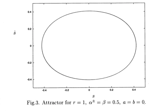
case
there are no exact solutions. Numerical solutions converge to the attractorin Fig.3 which is
a
closedcurve.
Thismeans
periodic solutionsare
stable.$\dot{s}$
$s$
Fig.3. Attractor for $r=1,$ $\alpha^{\pm}=\beta=0.5,$ $a=b=0$ .
Fig. 4 shows numerical results for $r=1,$ $\alpha^{\pm}=\beta=0$ and several initial
conditions. Solution
curves
converge to a point. Thismeans
the fixed point is theattractor. The steady state is stable.
$\dot{s}$
$s$
Fig. 5 shows the attractor for $r=1,$ $\alpha^{\pm}=\beta=0.5$. It is a closed
curve
inthe three-dimensional space. $u^{+}$ and $u^{-} \mathrm{r}\mathrm{e}\mathrm{p}\mathrm{r}\mathrm{e}\mathrm{S}\mathrm{e}\mathrm{n}\mathrm{t}_{\mathrm{S}}u^{+}(\frac{s(t)-1}{2}, t)$ and $u^{-}( \frac{1-s(t)}{2}, t)$,
respectively. $s,$ $u^{+}$ and $u^{-}$ are all unknowns of the ODE system which is derived
by the discretization of the PDE system. This
means our
approach enables toapproximate arbitrarily the original attractor of the PDE system in the functional
space.
$s$
Fig.5. Attractor in the solution space for $r=1,$ $\alpha^{\pm}=\beta=0.5,$ $a=b=0$.
5
Conclusion
In the papernumerical computation of attractors to
a
free boundary problems iscar-ried out. The problem considered here is a one-dimensional free boundary problem
with
some
parameters. This problem is of the type of a two-phase Stefanprob-lem. It is transformed into a fixed boundary problem by the fixed domain method.
Then, the spectral collocation method in space and time is applied for numerical
computation. From numerical results, attractors are found numerically for
some
values of parameters. Our next goal is investigation of Lyapunov exponents of the
Acknowledgement. Thiswork is partially supported by $\mathrm{c}_{\mathrm{r}\mathrm{a}\mathrm{n}\mathrm{t}-}\mathrm{i}\mathrm{n}$-Aidfor Scientific
Research($\mathrm{N}_{\mathrm{o}\mathrm{s}}$.
09440080
and 10354001). This work is alsoa
collaboration withCCSE ofJapan Atomic Energy Research Institute.
References
[1] T. Aiki, Global Attractors for Two-Phase Stefan Problems in One-Dimensional
Space, Abstract and Applied Analysis, 2(1-2), $\mathrm{p}\mathrm{p}.47- 66(1997)$.
[2] C. Canuto, et al., Spectral Methods in Fluid Dynamics, Springer-Verlag, New
York, 1988.
[3] H. Imai, Y. Shinohara and T. Miyakoda, Application of Spectral Collocation
Methods in Space and Time to Free Boundary Problems, ”Hellenic European
Research on Mathematic and Informatics ’94 (E.A. Lipitakis, ed.),” Hellenic
Mathematical Society, 2, $\mathrm{p}\mathrm{p}.781-786(1994)$.
[4] H. Imai, N. Ishimura and M. Nakamura, Convergence ofAttractors for the
Sim-plifiedMagnetic B\’enard Equations, European Journal of Applied Mathematics,
7, $\mathrm{p}\mathrm{p}.53- 62(1996)$.
[5] Y. Katano, T. Kawamura and H. Takami, Numerical Study of Drop Formation
from a Capillary Jet Using
a
General Coordinate System, ”Theoretical andApplied Mechanics,” Univ. Tokyo Press, $\mathrm{p}\mathrm{p}.3- 14(1986)$.
[6] Zhou W., H. Imai and M. Natori, Numerical Study of Convection with a
Free Surface by a Spectral Method, GAKUTO Internat. Ser. Math. Sci. Appl.,
![Fig. 2 shows these periodic solutions are not $\mathrm{s}\phi \mathrm{a}_{\mathrm{i}}\mathfrak{b}\mathrm{g}\mathrm{e}_{-}\backslash \mathrm{F}\emptyset$ ) $\mathrm{I}^{\cdot}\mathrm{s}\mathrm{f}_{\mathrm{k}}’\mathrm{g}\mathrm{h}\mathrm{t}$ ] $1\mathrm{y}\m](https://thumb-ap.123doks.com/thumbv2/123deta/6042315.1068768/6.892.161.760.92.508/periodic-solutions-mathrm-mathrm-mathrm-mathfrak-backslash-emptyset.webp)