Permanence of a single-species model with 2 stages (Dynamics of Functional Equations and Related Topics)

Permanence of asingle-species

model

with 2

stages

Ryusuke Kon

(_{今 隆助}

_,

_{[email protected]}

ne.jp)

1

Yasuhisa

Saito

(齋藤保久

, [email protected]

) 2

Yasuhiro Takeuchi

(_竹内康博

_,

_{y-takeuchi@eng.}

_Shizuoka

ac.jp

) 1

1

_Department

_of

Systems

Engineering,

Shizuoka

University

Hamamatsu,

432-8561, Japan

(静岡大学システム工学科)

2

_Department

_of

_Mathematical

_Sciences,

_{Osaka Prefecture}

University

Sakai, 599-8531, Japan

(

大阪府立大学数理工学科

)

1

Introduction

In thispaper, we considerpermanence of asingle-species model withtwo stages. The

model was proposed by Neubert and Caswe11[4] to consider the density dependence

effect to stage-structured systems. Their model has acomplex solution in the wide

range of the parameter space. Therefore, we give the conditions for permanence

to

ensure

that the species persists under such complex solutions. This paper is

organized as follows. In Section 2, we introduce asingle species model with two

stages. In Section 3, wegive the definition ofpermanence, and obtainboth sufficient

and necessary conditions for permanence of the model. The final section includes discussion and future problems.

2Stage-Structured Model

We consider permanence of the following stage-structured model:

$\mathrm{x}(t+1)=\mathrm{A}_{\mathrm{x}}\mathrm{x}(t)$ (1)

数理解析研究所講究録 1254 巻 2002 年 181-189

$\mathrm{x}(t)=(_{x_{2}(t)}x_{1}(t))\in \mathbb{R}_{+}^{2}:=\{(x_{1}, x_{2})\in \mathrm{R}^{2}$:

x:

_{$\geq 0,$}i _$=1,$

2}

$t\in \mathbb{Z}_{+}:=\{0,1,2, \ldots\}$

where

$\mathrm{A}_{\mathrm{x}}=\{$

$\sigma_{1}f_{1}(\mathrm{x}(t))\{1-\gamma f_{3}(\mathrm{x}(t))\}$

$\sigma_{2}f_{2}(\mathrm{x}(t))\phi f_{4}(\mathrm{x}(t)))$ . $\sigma_{1}f_{1}(\mathrm{x}(t))\gamma f_{3}(\mathrm{x}(t))$

Each $f_{i}$ : _{$\mathrm{R}^{2}+arrow(0,1](i=1, \ldots, 4)$},

which defines the way of density dependence,

is acontinuous function with $f_{i}(0,0)=1$, and the _{parameters satisfy} $0\leq\sigma_{1}\leq 1$,

$0\leq\sigma_{2}\leq 1,0\leq\gamma\leq 1$ and $0\leq\phi$. System (1) has two stages, namely, juvenile

and adult stages (see Fig.1). Population densities in the juvenile and adult stages at generation $t$ are denoted by _{$x_{1}(t)$} and

$x_{2}(t)$, respectively.

System (1) is the generalized _{version of the model introduced by Neubert and}

Caswell [4]. Putting $f_{i}(\mathrm{x}(t))=\exp[-(x_{1}(t)+x_{2}(t))]$

one

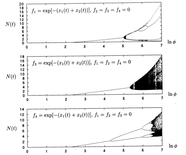
by one, they investigated

the dynamics of (1). Fig.2 shows some examplesof the complex solutions of System (1).

Figure 1: Life cycle of System (1). $\sigma_{1}fi$ and 02$f_{2}$ denote the fraction of

juveniles and adults which survive one generation, respectively. $\gamma f_{3}$ denotes

thefraction of thesurvivingjuveniles that matureto become adult. $\phi f_{4}$ is the

number of recruitedjuveniles byone adult individual.

3Permanence

The definition of permanence is given as follows

20 18 16 14 12 $N(t)$ $\mathrm{t}08$ 6 4 2 0 $\ln\phi$ $N(t)$ $\ln\phi$ 14 12 10 $N(t)$ $68$ $420$ $\ln\phi$

Figure 2: Bifurcation diagrams. The totalpopulationdensity$N(t)=x_{1}(t)+$

$x_{2}(t)$ is plotted for the orbit $\{\mathrm{x}(t)\}_{t\in\{1001,..,1050\}}$ with $\mathrm{x}(0)=(1,1)$. The

parametersare$\sigma_{1}=0.5$, $\sigma_{2}=0.1$ and$\gamma=0.1$. $\sigma_{1}\gamma\phi>(1-\sigma_{2})\{1-\sigma_{1}(1-\gamma)\}$

holds for $\ln\phi$ $>\ln 9.9\approx 2.293$.

$\mathrm{D}\mathrm{e}\mathrm{f}\mathrm{i}\mathrm{n}\mathrm{i}\mathrm{t}\mathrm{i}\dot{\mathrm{o}}\mathrm{n}1$

.

Let $N(t)= \sum_{i=1}^{2}x_{i}(t)$, which is a total population density.

Stage-structured system (1) is said to be permanent

_if

there exist $\delta>0$ and $D>0$ such

that

$\delta<\lim\inf N(t)tarrow\infty\leq\lim_{tarrow}\sup_{\infty}N(t)\leq D$

for

all $\mathrm{x}(0)\in \mathbb{R}_{+}^{2}$ with $N(0)>0$.

This definition implies that the following property is enough for permanence of

the stage-structured system (1): there exists a compact set $M\subset \mathbb{R}_{+}^{2}\backslash \{(0,0)\}$ such

that for all $\mathrm{x}(0)\in \mathbb{R}_{+}^{2}\backslash \{(0,0)\}$ there exists

a

_{$T=T(\mathrm{x}(0))>0$}

satisfying $\mathrm{x}(t)\in M$

for all $t\geq T$.

The definition ofpermanence

_seems

to be somewhat different from the

one

used

inotherliterature. That is, in Definition 1each$x_{i}$-axis does not havetobearepellor

and only _{the origin has to be. But thisproperty is appropriate for (1) because iffor}

all generation $t$ there is at least

one

stage in which

population is positive, we

can

conclude that the species _{survives. We must note that the variables,} $x_{1}$ and $x_{2}$, of

the stage-structured model (1) do not denote the population density of the different

species but the population density of the

same

species.

In order to_{prove the permanence of System (1),}

_we

_{consider the existence of the}

$\delta$ and _$D$ in Definition

1in turn.

3.1

Repellor

By using the following theorem, we consider the existence of the $\delta$ in Definition 1:

Theorem 2. (Hutson [3], Theorem 2.2) Let $(X, d)$ be a _metric space. _{Consider the}

system $F:Xarrow X$_{, where} $F$ is continuous. Assume that _$X$ is compact _{and that $S$} is a compact subset

_of

$X$ with empty interior. Let $S$ and$X\backslash S$ be$fo$ rward invariant.

Suppose that there is a continuous

_function

$P:Xarrow \mathbb{R}_{+}$, which is called an average

Liapunov_{function, satisfying the following conditions:} (a) $P(\mathrm{x})=0\Leftrightarrow \mathrm{x}\in S$,

(b)

$\sup_{t\geq 0}\lim_{\mathrm{y},\mathrm{y}\in X},\inf_{\mathrm{x},\backslash s},$

$\frac{P(F^{t}(\mathrm{y}))}{P(\mathrm{y})}>1$ $(\mathrm{x}\in S)$

.

Then $S$ is a repellor, that is, there is a compact set

$M\subset X\backslash S$ such that

for

all $\mathrm{x}\in X\backslash S$ there exists a _{$T=T(\mathrm{x})>0$} satisfying _{$F^{t}(\mathrm{x})\in M$}

for

all$t\geq T$.

We need the following lemma for the application of Theorem 2to the system

with uniformly ultimately bounded solutions:

Lemma 3. (Hutson [3], Lemma 2.1, Hofbauer et al. [2], Lemma 2.1) Consider the

system $F$ : _{$Xarrow X$}, where $F$ is continuous. Let $U$ be open with compact closure,

and suppose that $V$ is open and

forward

invariant, where $\overline{U}\subset\ddagger^{r}’\subset X$.

If

there

exists a $T=T(\mathrm{x})>0$ such that $F^{T}(\mathrm{x})\in U$

for

every $\mathrm{x}\in V$, then there eists

$a$

forward

invariant compact set $X_{0}\subset V$ such that there exists a _{$T_{0}=T_{0}(\mathrm{x})>0$}

satisfying $F^{\ell}(\mathrm{x})\in X_{0}$

for

all_{$t\geq T_{0}$}.

Applying Theorem 2to System (1) with $S=\{(0,0)\}$ and $P(\mathrm{x})=x_{1}+wx_{2}$,

where $w$ is apositive constant,

we

obtain the following theorem:

Theorem 4. Suppose that the solution

of

System (1) isuniformlyultimately bounded.

If

$\sigma_{1}\gamma\phi>(1-\sigma_{2})\{1-\sigma_{1}(1-\gamma)\}$, then System (1) is permanent.

Proof.

Since the solution of System (1) is uniformly ultimately bounded, Lemma 3

guarantees that there exists aforward invariant compact set $X$ such that all orbits

in $\mathbb{R}_{+}^{2}$ ultimately enter the $X$. Therefore, it is enough to consider the solutions in

$X$. First, we note that $\sigma_{1}\gamma\phi>(1-\sigma_{2})\{1-\sigma_{1}(1-\gamma)\}$ implies that $\sigma_{1}>0$, $\gamma>0$

and $\phi>0$.

Then

$X\backslash S$ is clearly forward invariant.

Let $w$ be apositive constant satisfying the following equation:

$w\sigma_{1}\{1+\gamma(w-1)\}=\phi+w\sigma_{2}$. (2)

Such apositive constant $w$ always exists. Indeed, the quadratic equation

$g(w)=\sigma_{1}\gamma w^{2}+\{\sigma_{1}(1-\gamma)-\sigma_{2}\}w-\phi$

is negative at $w=0$, that is, $g(0)=-\phi<0$.

Let us check the condition (b) in Theorem 2:

$\sigma$ $=$

$\sup_{t\geq 0}\lim_{\mathrm{y}\in X}\inf_{0\mathrm{y}(0,),\backslash s’}\frac{P(F^{t}(\mathrm{y}))}{P(\mathrm{y})}$

$=$ $\sup_{t\geq 0}\lim_{\mathrm{y}\in X}\inf_{0\mathrm{y}(0,),\backslash s’}\frac{P(F^{t}(\mathrm{y}))}{P(F^{t-1}(\mathrm{y}))}\ldots\frac{P(F^{2}(\mathrm{y}))}{P(F(\mathrm{y}))}\frac{P(F(\mathrm{y}))}{P(\mathrm{y})}$

$=$ $\sup_{t\geq 0}\lim_{\mathrm{y}\in X}\inf_{0\mathrm{y}(0,),\backslash s’}\prod_{i=0}^{t-1}[\frac{\sigma_{1}f_{1}(\mathrm{y}(i))\{1+\gamma(w-1)f_{3}(\mathrm{y}(i))\}y_{1}(i)}{y_{1}(i)+wy_{2}(i)}$

$+ \frac{\{\phi f_{4}(\mathrm{y}(i))+w\sigma_{2}f_{2}(\mathrm{y}(i))\}y_{2}(i)}{y_{1}(i)+wy_{2}(i)}]$

$=$ $\sup_{t\geq 0}\lim_{\mathrm{y}\in\lambda},\inf_{0\mathrm{y}(0,),\backslash s’}\prod_{i=0}^{t-1}[\sigma_{1}f_{1}(\mathrm{y}(i))\{1+\gamma(w-1)f_{3}(\mathrm{y}(i))\}$

$+(\begin{array}{l}i\ovalbox{\tt\small REJECT}\end{array})-w\sigma_{1}f_{1}(\mathrm{y}(i))\{1+\gamma(w-1)f_{3}(\mathrm{y})\}+\{\phi f_{4}(\mathrm{y}(i))+w\sigma_{2}f_{2}(\mathrm{y}(i))\}y_{2}(i)]$,

$y_{1}(i)+wy_{2}(i)$

where $\{\mathrm{y}(t)\}_{t\in \mathbb{Z}}+=\{(y_{1}(t), y_{2}(t))\}_{t\in \mathbb{Z}_{+}}$ is a solution of System (1) with

$\mathrm{y}=\mathrm{y}(0)$

and $F$ is defined as aright-hand side of (1). By Eq.(2), we have

$\lim_{\mathrm{y}(i)arrow(0,0)}[-w\sigma_{1}f_{1}(\mathrm{y}(i))\{1+\gamma(w-1)f_{3}(\mathrm{y}(i))\}+\{\phi f_{4}(\mathrm{y}(i))+w\sigma_{2}f_{2}(\mathrm{y}(i))\}]=0$ .

Furthermore,

we

havethe

boundedness

of$y_{2}(i)/(y_{1}(i)+wy_{2}(i))$. In fact, thefollowing

inequality holds for all $\mathrm{y}(i)\in X\backslash S$:

$\frac{y_{2}(i)}{y_{1}(i)+wy_{2}(i)}\leq\frac{(y_{1}(i)+wy_{2}(i))/w}{y_{1}(i)+wy_{2}(i)}=\frac{1}{w}$ .

Therefore, by the continuity of the $F$,

we

obtain

$\sigma=\sup_{\ell\geq 0}[\sigma_{1}\{1+\gamma(w-1)\}]^{\ell}$.

After

some

calculations, we

see

that $\sigma_{1}\gamma\phi>(1-\sigma_{2})\{1-\sigma_{1}(1-\gamma)\}$ implies that

$\sigma_{1}\{1+\gamma(w-1)\}>1$. Hence, the _{assumptions in Theorem 2hold.}

$\square$

3.2

Boundedness

Hereafter, we consider uniform _{ultimate boundedness of the solution ofSystem (1).}

Clearly, the

boundedness ensures

the existence of the D in Definition 1.

Theorem 5. Suppose that $\sigma_{1}\neq 1$ or

$\gamma$ $\neq 0$, and$\sigma_{2}\neq 1$.

If

one

of

_{$f_{1}(\mathrm{x})x_{1}$},

$f_{3}(\mathrm{x})x_{1}$

or $f_{4}(\mathrm{x})x_{2}$ is bounded to the above,

then the solution

of

System (1) is uniformly

ultimately bounded.

Proof

Let $\{\mathrm{x}(t)\}_{t\in \mathbb{Z}_{+}}$ be asolution of System (1).

First,

assume

that one of $f_{i}(\mathrm{x})x_{1}(i=1,3)$ is bounded to the above, _{that is,}

there exists

a

$K_{0}>0$ such that $x_{1}f_{i}(\mathrm{x})\leq K_{0}$ for all $\mathrm{x}\in \mathrm{R}_{+}^{2}$ and $i=1$

or

3. From

the second equation of (1), we have

$x_{2}(t+1)$ $=$ $\sigma_{1}f_{1}(\mathrm{x}(t))\gamma f_{3}(\mathrm{x}(t))x_{1}(t)+\sigma_{2}f_{2}(\mathrm{x}(t))x_{2}(t)$

$\leq$ $\sigma_{1}\gamma f_{i}(\mathrm{x}(t))x_{1}(t)+\sigma_{2}x_{2}(t)$

$\leq$ $\sigma_{1}\gamma K_{0}+\sigma_{2}x_{2}(t)$.

Since $\sigma_{2}\neq 1(0\leq\sigma_{2}<1)$, there exist $T>0$ and $K>0$ such that

$x_{2}(t)\leq K$

for all $t\geq T$. If$\sigma_{1}\neq 1$, then from the first equation of (1)

we have

$x_{1}(t+1)$ $=$ _{$\sigma_{1}f_{1}(\mathrm{x}(t))\{1-\gamma f_{3}(\mathrm{x}(t))\}x_{1}(t)+\phi f_{4}(\mathrm{x}(t))x_{2}(t)$} $\leq$ _{$\sigma_{1}x_{1}(t)+\phi x_{2}(t)\leq\sigma_{1}x_{1}(t)+\phi K$}

for $t\geq T$. If$\gamma\neq 0$, then similarly to the above we have

$x_{1}(t+1)$ $=$ $\sigma_{1}f_{1}(\mathrm{x}(t))\{1-\gamma f_{3}(\mathrm{x}(t))\}x_{1}(t)+\phi f_{4}(\mathrm{x}(t))x_{2}(t)$

$\leq$ $\{1-\gamma f_{3}(\mathrm{x}(t))\}x_{1}(t)+\phi x_{2}(t)\leq\{1-\gamma f_{3}(\mathrm{x}(t))\}x_{1}(t)+\phi K$

for $t\geq T$. Note that $\gamma\neq 0$ implies that $0<1-\gamma f_{3}(\mathrm{x}(t))<1$ for all $\mathrm{x}(t)\geq 0$.

These inequalities complete the proof of the first case.

Finally,

assume

that $f_{4}(\mathrm{x})x_{2}$ is bounded to the above, that is, there exists

a

$K_{0}>0$ such that $f_{4}(\mathrm{x})x_{2}\leq K_{0}$ for all $\mathrm{x}\in \mathbb{R}_{+}^{2}$. If $\sigma_{1}\neq 1$, then from the first

equation of (1) we have

$x_{1}(t+1)$ $=$ $\sigma_{1}f_{1}(\mathrm{x}(t))\{1-\gamma f_{3}(\mathrm{x}(t))\}x_{1}(t)+\phi f_{4}(\mathrm{x}(t))x_{2}(t)$ $\leq$ $\sigma_{1}x_{1}(t)+\phi f_{4}(\mathrm{x}(t))x_{2}(t)\leq\sigma_{1}x_{1}(t)+\phi I\iota_{0}$.

If$\gamma\neq 0$, then similarly to the above we have

$x_{1}(t+1)$ $=$ $\sigma_{1}f_{1}(\mathrm{x}(t))\{1-\gamma f_{3}(\mathrm{x}(t))\}x_{1}(t)+\phi f_{4}(\mathrm{x}(t))x_{2}(t)$

$\leq$ $\{1-\gamma f_{3}(\mathrm{x}(t))\}x_{1}(t)+\phi f_{4}(\mathrm{x}(t))x_{2}(t)\leq\{1-\gamma f_{3}(\mathrm{x}(t))\}x_{1}(t)+\phi K_{0}$

.

Then, there exist $T>0$ and $K>0$ such that

$x_{1}(t)\leq K$

for all $t\geq T$. From the second equation of (1), we have

$\mathrm{x}\mathrm{x}\{\mathrm{t}+1)$ $=$ $\sigma_{1}f_{1}(\mathrm{x}(t))\gamma f_{3}(\mathrm{x}(t))x_{1}(t)+\sigma_{2}f_{2}(\mathrm{x}(t))x_{2}(t)$

$\leq$ $\sigma_{1}\gamma x_{1}(t)+\sigma_{2}x_{2}(t)$

$\leq$ $\sigma_{1}\gamma K+\sigma_{2}x_{2}(t)$

for $t\geq T$. This completes the proof. $\square$

From the following theorem, we see that the boundedness of $f_{2}(\mathrm{x})x_{2}$ does not

imply uniform ultimate boundedness ofthe solution of (1).

Theorem 6. Assume that $f_{1}(\mathrm{x})=f_{3}(\mathrm{x})=f_{4}(\mathrm{x})=1$.

If

$\phi>1$, then System (1)

has an unbounded solution

Proof.

Suppose that allsolutionsofSystem (1) _{are bounded. Then there exist K} $>0$

and T $>0$ such that

$x_{1}(t)\leq K$

for all $t\geq T$. By (1), we have

$x_{1}(t+1)+x_{2}(t+1)$ $=$ $\sigma_{1}x_{1}(t)+\{\phi+\sigma_{2}f_{2}(\mathrm{x}(t))\}x_{2}(t)$

$\geq$ $\phi x_{2}(t)$.

Then $x_{2}(t+1)\geq$ $\mathrm{x}2(\mathrm{t}-\mathrm{x}2(\mathrm{t}+1)\geq$ $\mathrm{x}2(\mathrm{t}-K$ for $t$ $\geq T$. Since _$\phi>1$, it is

a

contradiction to the boundedness of the solution. ₀

By Theorems 4and 5, we obtain the following corollary:

Corollary 7. Assume that $\sigma_{1}\neq 1$ or $\gamma\neq 0$, and $\sigma_{2}<1$. Suppose that

one

of

$f_{1}(\mathrm{x})x_{1}$, $f_{3}(\mathrm{x})x_{1}$ _of$f_{4}(\mathrm{x})x_{2}$ is boundedto the above.

If

_{$\sigma_{1}\gamma\phi>(1-\sigma_{2})\{1-\sigma_{1}(1-\gamma)\}$},

then System (1) is permanent.

The following corollary is an immediate consequence ofTheorem 6:

Corollary 8. Assume that $f_{1}(\mathrm{x})=f_{3}(\mathrm{x})=f_{4}(\mathrm{x})=1$ .

If

_$\phi>1$, then System (1)

is not permanent.

4Discussion

and

Future

works

By Corollary 7, it is ensured that the system whose dynamics are shown in Fig.2 is

permanent if$\phi>9.9(\ln\phi>2.293)$.

The condition $\sigma_{1}\gamma\phi>(1-\sigma_{2})\{1-\sigma_{1}(1-\gamma)\}$ in Theorem 4has astrong

re-lationship with instability of the origin. In fact, _{Jacobian matrix at the origin of}

System (1) is given by

$A=(\begin{array}{lll}\sigma_{1}(1- \gamma) \phi\sigma_{1}\gamma \sigma_{2}\end{array})$,

and the eigenvalues Aofthe matrix satisfy $|\lambda|<1$ if and only if$\sigma_{1}\gamma\phi<(1-\sigma_{2})\{1-$

$\sigma_{1}(1-\gamma)\}$ (see Neubert and Caswe11[4]). Therefore, it is expected that under the

assumption of uniform ultimate boundedness System (1) is permanent if and only

ifthe origin is unstable. It is afuture work to show it

In Theorem 5we obtained sufficient conditions for uniform ultimate

bounded-ness

of the solution of (1). The sufficient conditions require the boundedness of

at least one of the functions $f_{1}(\mathrm{x})x_{1}$, $f_{3}(\mathrm{x})x_{1}$ or $f_{4}(\mathrm{x})x_{2}$. However, from the

anal-ogy between single-species models with stages and without stages, it is expected

that the solution of System (1) can be uniformly ultimately bounded

even

if all of

the $f_{1}(\mathrm{x})x_{1}$, $f_{3}(\mathrm{x})x_{1}$ and $f_{4}(\mathrm{x})x_{2}$

are

unbounded. In fact, the solution of the

fol-lowing single-species model with unbounded $f(N)N$ is clearly uniformly ultimately

bounded (a positive equilibrium of the system is globally stable, that is, all orbits

$\{N(t)\}_{t\in \mathbb{Z}_{+}}$ with $N(0)>0$ converge to apositive equilibrium point. This property

is proved by Theorem 1in Cull[l]$)$:

$N(t+1)=\phi Nf(N)$, $\phi>1$

$f(N)= \frac{1}{1+N^{1/2}}$.

To relax the condition in Theorem 5is afuture work.

System (1) can be easily extended to the system with $n$-stages. To consider the

permanence of the system is also afuture work.

References

[1] P. Cull, Local and global stability for population models. Biological cybernetics

54, 141-149 (1986).

[2] J. Hofbauer, V. Hutson and W. Jansen, Coexistence for systems governed by

difference equations of Lotka-Volterra type. Journal

_of

Mathematical Biology

25, 553-570 (1987).

[3] V. Hutson, Atheorem on average Liapunov functions.

Monatshefte fur

Mathe-matik 98, 267-275 (1984).

[4] M.G. Neubert and H. Caswell, Density-dependent vital rates and their

pop-ulation dynamic consequences. Journal

_of

Mathematical Biology 41, 103-121

(2000