Population Aging, Sustainability of Public
Debt, and Endogenous Growth
journal or
publication title
経済学論究
volume
68
number
3
page range
75-98
year
2014-12-20
URL
http://hdl.handle.net/10236/13407
Population Aging,
Sustainability of Public Debt,
and Endogenous Growth
Ken Tabata
∗This paper examines how population aging influences the sustainability of public debt in an overlapping generations model with unfunded social security. We show that population aging increases the government’s risk of bankruptcy and negatively affects economic growth when the population growth rate is sufficiently low. We also show that social security reform reduces the government’s risk of bankruptcy and positively affects economic growth.
Ken Tabata
JEL:E62, H55, H63, O40
Keywords:population aging, social security, public debt, economic growth
1 Introduction
This paper develops an overlapping generations model of growth and public debt according to the model suggested by Br¨auninger (2005), and then uses this framework to analyze the economic impact of population aging and social security reform. The situation considered here is that an aging population causes a heavy burden of social security payments, while social security tax alone would not be sufficient to finance such payments fully. Public debt is introduced in order to supplement this
* Address: School of Economics, Kwansei Gakuin University, 1-155 Uegahara Ichiban-cho, Nishinomiya 662-8501, Hyogo, Japan;
balance. In such a situation, we examine how population aging influences the sustainability of public debt and economic growth. Furthermore, the economic impact of social security reform will also be examined.
The present analysis is motivated by two important issues in Japan, population aging and government budget deficits. Population aging is triggered by a rise in life expectancy and a decline in the fertility rate. According to demographic projections by the United Nations Population Division, the old-age dependency ratio (the share of the total population aged 65 and over) in Japan is expected to grow from 19.7% in 2005 to 37.7% in 2050, while the working population share (the share of the total population aged 15–64) is expected to decline from 66.4% in 2000 to 51.1% in 2050. 1) In addition, the public debt in Japan exploded after the collapse of the “bubble economy”. According to OECD Economic Outlook 2006, the debt/GDP ratio in Japan increased from 74.7% in 1993 to 177.6% in 2007. Because the Japanese public pension scheme is based on a pay-as-you-go pension scheme, population aging leads to a greater burden of social security payments on younger generations. In addition, as stressed by Ono (2003), because the social security payments are partly funded by the state budget, government deficits and social security finance are closely related to each other. Therefore, this paper constructs a growth model that explicitly incorporates unfunded social security and public debt, and analyzes how population aging and social security reform influence the sustainability of public debt. Note that population aging is a common feature of developed countries. Many developed countries also employ pay-as-you-go pension schemes. Moreover, most developed countries have experienced continual budget deficits since the mid 1970s. Therefore, the implications of this paper
1) Source: The World Population Prospects: The 2006 Revision Population Database.
are also applicable to many other developed countries.
Existing studies such as Pecchenino and Polland (1997), Pecchenino and Utendorf (1999), and Futagami and Nakajima (2001) analyzed unfunded social security and population aging in economic growth models. However, these studies did not consider the issue of public debt explicitly. Previous studies such as Chalk (2000), Br¨auninger (2005) and Yakita (2008) examined the sustainability of public debt using an overlapping generations model. For example, Br¨auninger (2005) employed a Romer (1986) type endogenous growth model and showed that there is a critical deficit–GDP ratio. If the deficit–GDP ratio is below the critical level, there exists a stable steady-growth path. However, if the deficit–GDP ratio is above the critical level, the bond-financed deficit is not sustainable. However, these studies do not consider the issue of social security explicitly. To my knowledge, Gertler (1997) and Ono (2003) are two exceptional analytical studies that explicitly considered both the issues of social security and public debt. Gertler (1997), who modified the Blanchard (1985) and Weil (1989) framework, analyzed social security as financed by public debt. Ono (2003) analyzed a social security policy with public debt using a Diamond (1965) type overlapping generations model. However, these studies employed neoclassical growth models. Thus they cannot examine the growth effects of population aging and social security reform. Moreover, they did not focus their attention on the sustainability of public debt. Therefore, this paper extends a Br¨auninger (2005) type endogenous growth model by introducing unfunded social security and examines how population aging and social security reform influence economic growth and the welfare of agents.
The main findings of this paper are as follows. First, population aging caused by the decline in the population growth rate increases the government’s risk of bankruptcy, while a reduction in the old-age
pension benefit contributes to the sustainability of public debt. Second, population aging caused by the decline in the population growth rate negatively affects economic growth when the population growth rate is low, but it positively affects economic growth when the population growth rate is high. In addition, a reduction in the old-age pension benefit positively affects economic growth.
This paper is organized as follows. In Section 2, we present the basic model. Section 3 shows how population aging or a reduction in the old-age pension benefit influences the sustainability of public debt. In Section 4, we examine how population aging or a reduction in the old-age pension benefit influences the long-run growth rate of the economy. Finally, Section 5 provides concluding remarks.
2 The model
2.1 Basic setup
We consider a one-sector, endogenous growth model with unfunded social security. In each period t, a new generation, called generation t, is born and is composed of a continuum of Nt> 0 units of identical agents. The population growth rate is assumed to be constant at n∈ (−1, ∞) and satisfies Nt = (1 + n)Nt−1. Agents in this economy live for two periods, youth and old age. In each period t, there exist only two generations, the active working young and the retired old. Therefore, the share of old dependents relative to the young working population in period t is given by Nt−1
Nt =
1
1+n. Thus, population aging would be
triggered if there were a decrease in the population growth rate n. Agents derive utility from their own consumption in both youth and old age. Thus, the lifetime utility of the agent in generation t is expressed as:
ut= ln c1,t+ β ln c2,t+1, (1)
where c1,t and c2,t+1 denote the consumption when young and old, and
β is a time discount rate.
In youth, each agent is endowed with one unit of labor, works inelastically, and obtains wage income. An agent in generation t divides his or her wage income wt between his or her own current consumption
c1,t, savings st, and the payment of social security taxes τtwt, where
τt is the rate of social security tax levied on wage income. In old age, agents retire and consume their returns on savings (1 + rt+1)st and social security benefits zt+1.
Thus, the lifetime budget constraints of the agent in generation t are:
c1,t+ st= (1− τt)wt, (2)
c2,t+1= (1 + rt+1)st+ zt+1. (3) By maximizing (1), subject to (2) and (3), we obtain:
st= β 1 + β(1− τt)wt− 1 1 + β zt+1 1 + rt+1 . (4)
This saving equation states that higher social security benefits zt+1 and tax rate τt imply lower savings.
Each firm has constant returns-to-scale technology, and the aggregate production function is expressed as Yt = F (Kt, EtNt), where Yt, Kt, and Nt denote the aggregate levels of output, physical capital, and labor input, respectively. Et represents labor productivity, which is assumed to be driven by Romer-type spillovers that emanate from accumulated investment per worker. In order to ensure the existence of a long-run growth path, it is assumed that Et takes a particular form as follows:
Et = a1KNt
t =
kt
parameter. Representing the production function in effective per capita terms, ˆyt= f ( ˆkt), where ˆyt≡ Yt/EtNt, ˆkt≡ Kt/EtNt, and noting that
ˆ
yt = f (a) and ˆkt = a hold, we obtain the optimal condition for a representative firm as: ρt= f0(a) = ρ, (5) wt= » f (a)− f0(a)a a – kt= ¯wkt, (6) where ρ≡ f0(a) and ¯w≡ f (a)−fa0(a)a. Because the market for capital is competitive, the following arbitrage condition holds:
1− δ + ρt+1= 1 + rt+1= 1 + r, (7) where δ is the depreciation rate of capital. Because ρt+1 is constant at
ρ, the rate of return on savings rt+1 is also constant at r.
The government in this economy can impose a social security tax, τt, on wages. Moreover, it can issue public debt with a one-period maturity in order to finance social security payments. The government funds the expenditure of social security and the repayment of debt with tax receipts and with the revenue from the newly issued debt. Thus the government budget constraint in period t is given by Dt+1+τtwtNt= ztNt−1+(1+rt)Dt. With regard to the left-hand side, Dt+1 is the revenue from debt issue, while τtwtNt is the revenue from social security tax. With regard to the right-hand side, ztNt−1 represents the social security payments, while
Dt is the value of public debt maturing during period t, and rt, is the rate of return. Dividing both sides by Nt, we obtain:
(1 + n)dt+1+ τtwt=
zt
1 + n+ (1 + rt)dt, (8)
where dt≡DNt
t.
We assume that the government provides unfunded social security using a defined benefit scheme. Under the defined benefit scheme, there are two forms of social security payments. One is a lump sum transfer
where the payments for old agents in generation t−1 are a fixed constant
zt= z. The other is a transfer based on a replacement rate for wages, where the payments for old agents in generation t− 1 are calculated using a replacement rate for the next generation’s wages zt= φwt, where
φ ∈ [0, 1) denotes the replacement ratio. In the theoretical analysis,
the former (a lump sum) payment scheme is the general assumption. However, in the real world, many developed countries employ the latter payment scheme characterized by a strong link to current wages. In order to maintain the living standards of the elderly, the pension benefits are adjusted taking into account not only price changes (i.e., price indexation) but also wage changes (i.e., wage indexation). For example, in Japan, the pension benefit level of a salaried worker is set to exceed approximately 50% of the wages of the current working population. Therefore, the replacement ratio is about 50%. In our paper, we focus upon the role of wage indexation and assume that the payments for old agents in generation t− 1 are calculated using a replacement rate for the next generation’s wages zt = φwt. Existing studies such as Meier (2000) and Brooks (2002) also employ an analogous assumption. 2)
We also assume that the government employs the following fiscal rule concerning newly issued debt: Dt+1− Dt= ψYt, where Dt+1− Dt expresses the budget deficit in period t. The government borrows a specified fraction ψ of national income Yt and tries to maintain the budget deficit–GDP ratio constant at ψ. 3) This type of fiscal policy
2) Another reason for the assumption zt = φwt is purely technical. This
assumption makes the analysis of this paper employing an endogenous growth model with unfunded social security easier.
3) An alternative fiscal rule is that the government sets a constant tax rate, τ , and issues public debt to finance the remaining social security expenditure and the repayment of debt. Provided that this alternative fiscal rule is employed, the analytical property of the model is mostly unchanged.
is employed in the EU and other OECD countries. Existing studies such as Br¨auninger (2005) and Yakita (2008) also employ an analogous assumption. Dividing both sides by Nt leads to:
(1 + n)dt+1= dt+ ψyt, (9)
where yt≡ NYtt, and the relations yt= f (a)kt= ( ¯w + ρ)kt hold.
Under these social security and fiscal policies, the tax rate is adjusted endogenously to maintain the social security expenditure and the repayment of public debt. From (5)–(9) and zt = φwt, the social security tax rate τt is given by:
τt= φ 1 + n+ r ¯ wxt− ψ “ 1 + ρ ¯ w ” , (10)
where xt≡ dktt. Equation (10) states that a lower population growth rate n, a higher replacement ratio φ, and a higher debt–capital ratio
xt imply a higher social security tax rate.
Now let us consider the market equilibrium conditions. Noting that an arbitrary opportunity exists between a real asset and bond, we can set the market clearing condition for capital as: Kt+1+ Dt+1= stNt, which expresses the equality of the total savings by young agents in generation t, stNt, to the sum of the stocks of aggregate physical capital and aggregate public debt. Dividing both sides by Nt leads to:
(1 + n)(kt+1+ dt+1) = st. (11)
The commodity market clears automatically according to Walras’s law.
2.2 Equilibrium
This subsection characterizes the competitive equilibrium allocation of the economy. By inserting yt = ( ¯w + ρ)kt into (9), we obtain the dynamic evolution of the debt–labor ratio, dt, as:
dt+1 dt = 1 1 + n » 1 + ψ( ¯w + ρ)1 xt – ≡ dg(xt). (12)
Let us denote the right-hand side of (12) as dg(xt). Moreover, by inserting (4)–(7), (10),(12) and zt= φwtinto (11), we obtain the dynamic evolution of the capital–labor ratio, kt, as:
kt+1 kt = 1 1 + n + 1 1+β φ ¯w 1+r β 1 + β(1− φ 1 + n) ¯w− (1 + β 1 + βr)xt− ψ( ¯w + ρ) 1 + β ff ≡ kg(xt). (13)
Let us denote the right-hand side of (13) as kg(xt). The dynamics of the model are completely described by these two difference equations. Because the evolutions of the debt–labor ratio, dt, and the capital–labor ratio, kt, depend upon the debt–capital ratio, xt, the evolution of xt is given by: xt+1 xt = dt+1 dt kt+1 kt =dg(xt) kg(xt) . (14)
Therefore, the steady-state equilibrium is characterized by the conditions that xt+1= xt= x or:
1 + g = dg(x) = dk(x). (15)
From (12) and (13), in the steady-state equilibrium, the state variable
kt and dt grow at the same rate g. Hereafter, we denote the path on which the state variable kt and dt grow as the same rate as the balanced growth path, and denote the growth rate g defined in equation (15) as the balanced growth rate.
3 Steady state
In this section, we examine the existence and the stability of the steady-state equilibrium. Then, we also examine how population aging or a reduction in the old-age pension benefit influences the sustainability of public debt.
3.1 Existence of the steady-state equilibrium
This subsection examines the existence of the steady-state equilibrium. As discussed in Section 2-2, the steady-state equilibrium is characterized by equation (15). From (12) and (13), equation (15) is rewritten as:
LH(x; n, φ) = RH(x), (16) where LH(x; n, φ) ≡ 1 + n 1+n+ 1 1+β φ ¯w 1+r β 1+β(1− φ 1+n) ¯w−(1+ β 1+βr)xt− ψ( ¯w+ρ) 1+β ff , and RH(x)≡ 1 + ψ( ¯w + ρ)1 xt .
From (16), we can easily confirm that ∂LH∂x < 0, limx→0LH(x) <∞,
limx→∞LH(x) =−∞, ∂RH∂x < 0, limx→0RH(x) =∞, limx→∞RH(x) > 0. In addition, regarding the left-hand side of (16), ∂LH
∂n > 0 and ∂LH
∂φ < 0 hold. To stress these relationships, we denote the left-hand side of (16) as LH(x; n, φ) and the right-hand side of (16) as RH(x) respectively. Figure 1 illustrates LH(x; n, φ) and RH(x) for given values of n and φ. 4) From (16), regarding the existence of the steady-state
equilibrium, we obtain the following proposition.
Proposition 1 Regarding the existence of the steady-state equilibrium,
the following statements hold.
(1) There is a critical population growth rate ˆn. If the population growth rate n is above the critical level n > ˆn, then there are
4) Following Br¨auninger (2005) and Yakita (2008), we mainly focus our attention on the regions where the debt–capital ratio xt is positive. However, this
is only for clarity of explanation. Even if we consider the case where the debt–capital ratio xt is negative, the results of this paper do not change at
Figure 1: Existence of equilibria LH(x; n.φ),RH(x) x 0 x1 RH(x) LH(x; n, φ) x2 1 E1 E2 E 1 E 2 x1 xM x2
two steady states, E1 and E2, where E1 is characterized by a
lower debt–capital ratio x1, and E2 is characterized by a higher
debt–capital ratio x2. In these steady states, 0 < x1< x2, dx1
dn < 0
and dxdn2 > 0 hold. If the population growth rate n is below the critical level n < ˆn, then there is no steady state. Only at n = ˆn is there a unique steady-state equilibrium.
(2) There is a critical replacement ratio ˆφ. If the replacement ratio φ is below the critical level φ < ˆφ, then there are two steady states, E1 and E2 where E1 is characterized by a lower debt–capital ratio
x1, and E
2 is characterized by a higher debt–capital ratio x2. In
these steady states, 0 < x1< x2, dxdφ1 > 0 and dxdφ2 < 0 hold. If the replacement ratio φ is above the critical level φ > ˆφ, then there is no steady state. Only at φ = ˆφ is there is a unique steady-state equilibrium.
The proof of Proposition 1 is given in Appendix A. Proposition 1-1 indicates that there exist two steady states, E1 and E2, when the
population growth rate n is sufficiently high. As described in Figure 1, the decline in the population growth rate n shifts the function LH(x) downwards and thus increases the value of x1, and lowers the value of
x2. However, if the population growth rate n declines further, LH(x) and RH(x) may not intersect any more. In this case, there is no steady state. Therefore, there is a critical population growth rate ˆn. If the
population growth rate n is above the critical level n > ˆn, then there
are two steady states. However, if the population growth rate n is below the critical level n < ˆn, then there is no steady state.
Proposition 1-2 also indicates that there exist two steady states, E1
and E2, when the replacement ratio φ is sufficiently low. As again
described in Figure 1, an increase in the replacement ratio φ shifts the function LH(x) downwards and thus increases the value of x1 and lowers the value of x2. However, if the replacement ratio φ is increased
further, LH(x) and RH(x) may not intersect any more. In this case, there is no steady state. Therefore, there is a critical replacement ratio
ˆ
φ. If the replacement ratio φ is below the critical level φ < ˆφ, then
there are two steady states. However, if the replacement ratio φ is above the critical level φ > ˆφ, then there is no steady state.
3.2 Stability of the steady-state equilibrium
This subsection examines the stability of the steady-state equilibrium. As discussed in Section 2-2, the dynamics of the model are completely described by equations (12), (13) and (14). Figure 2 depicts equations (12) and (13), when there exist two steady states, E1 and E2. Figure
3 depicts equation (12) and (13), when there is no steady state. We denote the right-hand side of equation (12) as dg(xt), and the right-hand
side of equation (13) as kg(xt), respectively. From (12), (13) and (14), regarding the stability of the steady-state equilibrium, we obtain the following proposition.
Proposition 2 . Suppose there are two steady states, E1 and E2, and
the steady state E1 characterized by a lower debt–capital ratio, x1, is
locally stable, whereas the steady state E2 characterized by a higher
debt–capital ratio, x2, is unstable.
The proof of Proposition 2 is given in Appendix B. The intuition of proposition 2 is explained as follows. From Figure 2, the relation
kg(xt) > dg(xt) holds when x1 < xt< x2. In this region, because the capital–labor ratio kt grows faster than the debt–labor ratio dt, the debt–capital ratio xt decreases monotonically (i.e., xxt+1t < 1). However, when xt< x1 or xt> x2, the relation kg(xt) < dg(xt) holds. In these regions, the debt–labor ratio dt grows faster than the capital–labor ratio
Figure 2: Two steady-states dg(xt),kg(xt) x 0 x1 dg(xt) kg(xt) x2 1 1+n E1 E2
kt, and the debt–capital ratio xt increases monotonically (i.e., xxt+1
t > 1).
Therefore, if the initial debt–capital ratio x0 is below the critical level
x2, the debt–capital ratio gradually converges to the steady state x1. Thus steady state E1 characterized by the lower debt–capital ratio x1
is locally stable. However, if the initial debt–capital ratio x0 is above
the critical level x2, the debt–capital ratio xt increases monotonically, and the level of the capital–labor ratio kt decreases from (13) and will go to zero within a finite number of periods. Once the level of the capital–labor ratio kt becomes zero, there is no commodity in the economy, so the value of government debt vanishes. Thus such a situation can be regarded as government bankruptcy.
Figure 3 illustrates the case where there exists no steady state. In this case, as shown in Figure 3, the relation dg(xt) > kg(xt) holds for all xt > 0. Thus, regardless of the initial debt–capital ratio x0, the
debt–capital ratio xt increases monotonically (i.e., xxt+1
t > 1), and the
level of the capital–labor ratio kt decreases from (13) and goes to zero within a finite number of periods. Hence, the economy always rides on the path to bankruptcy.
Summarizing the results obtained in Sections 3-1 and 3-2, we obtain the following results.
Result 1 Regarding the sustainability of the bond-financed deficit, the
following statements hold.
(1) The bond-financed deficit is sustainable when the population growth rate n is sufficiently high to satisfy n > ˆn and the initial debt–capital ratio x0 is sufficiently low to satisfy x0< x2.
(2) The bond-financed deficit is sustainable when the replacement ratio φ is sufficiently low to satisfy φ < ˆφ and the initial debt–capital ratio x0 is sufficiently low to satisfy x0< x2.
Figure 3: No steady-state dg(xt),kg(xt) x 0 dg(xt) kg(xt) 1 1+n
These results are summarized as follows. The bond-financed deficit is not sustainable when there is no steady state. From Proposition 1, the existence of the steady-state equilibrium is assured when the population growth rate n is sufficiently high to satisfy n > ˆn or the replacement
ratio φ is sufficiently low to satisfy φ < ˆφ. However, these are not sufficient conditions for the sustainability of public debt. As shown in Proposition 2, the initial debt–capital ratio x0 plays a crucial role. In
order to prevent government bankruptcy, the initial debt–capital ratio
x0 must be sufficiently low to satisfy x0< x2. Therefore, a sufficiently
high population growth rate n, a sufficiently low replacement ratio φ and a sufficiently low initial debt–capital ratio x0 are sufficient conditions
for the sustainability of public debt.
3.3 Population aging and social security reform
In this subsection, we examine briefly how population aging caused by the decline in the population growth rate n influences the sustainability
of public debt. We also examine how a reduction in the old-age pension benefit caused by the decline in the replacement ratio φ influences the sustainability of public debt.
Let us first examine the effect of population aging. From Proposition 1-1, a lower population growth rate n is less likely to satisfy the condition
n > ˆn, which ensures the existence of the steady-state equilibrium.
Moreover, a lower population growth rate n decreases the critical value of x2, as shown in Proposition 1-1, and shrinks the regions of the
initial debt–capital ratio x0 where the economy can ride on the balanced
growth path. Therefore, population aging caused by the decline in the population growth rate n increases the government’s risk of bankruptcy by enlarging the burden of social security expenditure and the repayment of public debt.
Next, let us consider the effect of a reduction in the old-age pension benefit. From Proposition 1-2, a lower replacement ratio φ is more likely to satisfy the condition φ < ˆφ, which ensures the existence of
steady-state equilibrium. Moreover, a lower replacement ratio φ increases the critical value of x2 as shown in Proposition 1-2 and expands the
region of the initial debt–capital ratio x0 where the economy can ride on
the balanced growth path. Therefore, a reduction in the old-age pension benefit caused by the decline in the replacement ratio φ contributes to the sustainability of public debt by mitigating the burden of social security expenditure and the repayment of public debt.
4 Long-run growth
Section 3 shows that population aging increases the government’s risk of bankruptcy, while a reduction in the old-age pension benefit contributes to the sustainability of public debt. In this section, we focus on the case where the economy is in a stable steady-state equilibrium
E1, and we analyze the long-run growth effects of these policies. We
examine how population aging caused by a decline in the population growth rate n influences the balanced growth rate g. We also examine how a reduction in the old-age pension benefit caused by the decline in the replacement ratio φ influences the balanced growth rate g.
4.1 Population aging
This subsection examines the long-run growth effect of population aging caused by a decline in the population growth rate n. As shown in Section 2-2, the balanced growth rate g is described by (13), (15) and (16). However, because the debt–capital ratio, x1, is determined by a
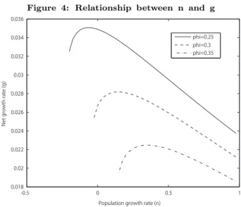
somewhat complicated form of the implicit function shown in (16), it is difficult to investigate the growth effect of n analytically. Therefore, in this subsection, we provide some numerical examples. In the numerical simulation, we specify the production function as Yt= AKtα(EtNt)1−α. Figure 4 depicts numerical examples of the relationship between the population growth rate n and the balanced growth rate g under alternative values of φ. The parameters used in the baseline simulations are given in footnote 5.5)The figures show that there is a hump-shaped relationship between the population growth rate n and the balanced growth rate
g.6) These results indicate that the growth effect of population aging caused by the decline in the population growth rate n is positive when the population growth rate n is high but that it could be negative when the population growth rate is low. These results are intuitively explained as follows.
5) α = 0.25, A = 16, a = 1, δ = 1, ψ = 0.03, β = 1, n = 0,φ = 0.3.
6) Note that the balanced growth rate is defined only when the population growth rate n is sufficiently high to satisfy n > ˆn. For example, the φ = 0.3
line in Figure 4 suggests that the critical population growth rate when φ = 0.3 is −0.025.
Figure 4: Relationship between n and g -0.5 0 0.5 1 0.018 0.02 0.022 0.024 0.026 0.028 0.03 0.032 0.034 0.036
Population growth rate (n)
Net gr
owth rate (g)
phi=0.25 phi=0.3 phi=0.35
Equation (13) indicates that the decline in the population growth rate
n has two negative effects and one positive effect on capital accumulation.
The first negative effect is the “tax increase effect”. Equation (10) implies that the decline in the population growth rate n positively affects the tax rate τ in the following two ways. First, the decline in
n increases the dependency ratio 1
1+n, which positively affects the tax
rate. Second, the decline in n increases the debt–capital ratio x1 as
shown in Proposition 1-1, which positively affects the tax rate. These two positive effects of the decline in n on τ decrease the net labor earnings and savings of agents and thus negatively affect the capital accumulation. The second negative effect is the “substitution effect from physical capital to public debt”. Proposition 1-2 shows that the decline in n increases the debt–capital ratio x1. This increase in the debt–capital ratio implies a shift in savings from physical capital to public debt. Thus this substitution effect negatively affects the capital accumulation.
The one positive effect is the “antidissolving effect”. From (11), the decline in n increases the ratio of old to young in the population, which mitigates the dissolving of savings into a larger workforce st
1+n. Thus
this antidissolving effect positively affects the capital accumulation From (13) and (16), it is easy to guess that the effect of the decline in n is likely to be negative when n is extremely small (i.e., n→ −1). Because the ratio of old to young in the population is already large, the positive dissolving effect caused by the decline in n becomes negligible. However, because the social security tax rate is already high because of the high dependency ratio and the high debt–capital ratio, any increase in social security tax caused by the decline in the population growth rate
n provides a considerable negative impact upon capital accumulation.
Therefore, when n is extremely small, the negative tax reduction effect and substitution effect are likely to dominate the positive antidissolving effect. On the other hand, the effect of the decline in n is likely to be positive when n is extremely large (i.e., n→ ∞). Because the ratio of old to young in the population is already small, the positive antidissolving effect caused by the decline in n becomes more crucial. However, because the social security tax rate is already low because of the low dependency ratio and the low debt–capital ratio, any increase in social security tax caused by the decline in the population growth rate
n provides a fairly small negative impact upon capital accumulation.
Therefore, when n is extremely large, the positive antidissolving effect is likely to dominate the negative tax reduction effect and the substitution effect.
Therefore, these numerical examples suggest that population aging caused by the decline in the population growth rate may not only increase the government’s risk of bankruptcy but also decrease the rate of capital accumulation and the balanced-growth rate when the population growth rate n is sufficiently low.
4.2 Social security reform
This subsection examines the long-run growth effect of a reduction in the old-age pension benefit caused by a decline in the replacement ratio φ. The balanced growth rate g is again described by (13), (15) and (16). From (13), (15) and (16), regarding the effect of φ on g, we obtain the following proposition.
Proposition 3 . In the stable steady state E1, dφdg < 0 holds.
The proof of Proposition 3 is simple. By differentiating (13) with respect to φ and noting dx1
φ > 0 from Proposition 1-2, we can easily confirm that the relation dgdφ < 0 holds. Proposition 3 shows that the
decline in the replacement ratio φ increases the balanced growth rate. Equation (13) indicates that the decline in the replacement ratio φ has three positive effects on capital accumulation. The first positive effect is the “tax reduction effect”. Equation (10) implies that the decline in
φ negatively affects the tax rate τ in the following two ways. First, the
decline in φ decreases the level of social security expenditure, which negatively affects the tax rate. Second, the decline in φ lowers the debt–capital ratio x1 as shown in Proposition 1-2, which negatively affects the tax rate. These two negative effects of the decline in φ on τ increase the net labor earnings and savings of agents and thus positively affect the capital accumulation. The second positive effect is the “substitution effect from public debt to physical capital”. Proposition 1-2 shows that the decline in φ lowers the debt–capital ratio x1. This
reduction in the debt–capital ratio implies a shift in savings from public debt to physical capital. Thus this substitution effect positively affects the capital accumulation. The third positive effect is the “incentive effect”. The decline in φ implies the reduction in the old-age pension benefit. Thus, it motivates agents to save more for their old age, which
positively affects the capital accumulation.
Therefore, we can confirm that a reduction in the old-age pension benefit caused by the decline in the replacement ratio φ not only contributes to the sustainability of public debt but also increases the rate of capital accumulation and the balanced-growth rate.
5 Concluding remarks
This paper examined how population aging influences the sustainability of public debt in an overlapping generations model with unfunded social security. We showed that population aging increases the government’s risk of bankruptcy and negatively affects economic growth when the population growth rate is sufficiently low. We also showed that social security reform reduces the government’s risk of bankruptcy and positively affects economic growth.
References
[1] Blanchard, O.J.,(1985). “Debt, deficits, and finite horizons”, Journal
of Political Economy 93, 223–247.
[2] Br¨auninger, M.,(2005). “The budget deficit, public debt, and endogenous
growth”, Journal of Public Economic Theory 7, 827–840.
[3] Brooks, R.J.,(2002). “Asset-market effects of the baby boom and
social-security reform”, American Economic Review 92, 402–406.
[4] Chalk, N.A.,(2000). “The sustainability of bond-financed deficits: an
overlapping generations approach”, Journal of Monetary Economics 45, 293–328.
[5] Diamond, P.A.,(1965). “National Debt in a Neoclassical Growth Model”,
American Economic Review 55, 1126–1150.
[6] Futagami, K. and T. Nakajima,(2001). “Population aging and economic
[7] Gertler, M.,(1997). “Government debt and social security in a life cycle economy”, NBER Working Paper No. 6000.
[8] Meier, V.,(2000). “Time Preference and International Migration, and
Social Security”, Journal of Population Economics 13, 127–146.
[9] Ono,T.,(2003). “Social Security Policy with Public Debt in an Aging
Economy”, Journal of Population Economics16, 363–387.
[10] Pecchenino, R. and P. Pollard,(1997). “The effect of annuities, bequests
and aging in an overlapping generations model of endogenous growth”,
Economic Journal 107, 26–46.
[11] Pecchenino, R. and K. Utendorf,(1999). “Social security, social welfare
and the aging population”, Journal of Population Economics 12, 607–623.
[12] Romer, P.M.,(1986). “Increasing returns and long-run growth”, Journal
of Political Economy 94, 1002–1037.
[13] Weil, P.(1989). “Overlapping families of infinitely-lived agents”, Journal
of Public Economics 38, 410–421.
[14] Yakita, A.(2008). “Sustainability of public debt, public capital formation,
and endogenous growth in an overlapping generations setting”, Journal
Appendix A: Proof of Proposition 1
We denote the value of x such that satisfies the condition ∂LH
∂x = ∂RH
∂x as xM. From (16), we can easily confirm that
xM = (LHRH1LH2 3)1/2 where LH1 ≡ 1+n+1+n1 1+β
φ ¯w
1+r
, LH3 ≡ 1 + 1+ββ r
and RH2 ≡ ψ( ¯w + ρ). Since limx→0LH(x) < limx→0RH(x) and limx→∞LH(x) < limx→∞RH(x), the following three cases might occur, RH(xM) < LH(xM), RH(xM) = LH(xM), and RH(xM) > LH(xM). We denote RH(xM) < LH(xM) as case1, RH(xM) = LH(xM) as case 2, and RH(xM) > LH(xM) as case 3 respectively.
If RH(xM) < LH(xM) (i.e. case 1), as shown in Figure 1, the function RH(x) and LH(x) have necessarily two intersections, so there are two steady-states, x1 and x2. If RH(xM) = LH(xM) (i.e. case 2), the function RH(x) and LH(x) are just tangent at xM and there is a unique steady-state. If RH(xM) > LH(xM) (i.e. case 3), RH(x) and
LH(x) do not intersect and therefore there is no steady-state.
Now notice that ∂LH∂n > 0. Hence, an increase in population growth
rate n increases LH(x). Therefore, if the population growth rate n is sufficiently high to satisfy n > ˆn, the situation called case 1 occurs and
there will be two steady-states, x1 and x2. However, if the population growth rate n is sufficiently low to satisfy n < ˆn, there will be no
steady-state. Then critical value of ˆn is defined as the value of n which
yields the situation called case 2.
In addition, by differentiating (16) with respect to n, we obtain
dx dn=− ∂LH ∂n ∂LH ∂x − ∂RH ∂x . Since ∂LH ∂n > 0 and 0 > ∂LH ∂x > ∂RH ∂x at x 1 (0 > ∂RH ∂x > ∂LH ∂x at x 2) as
shown in Figure 1, we can easily confirm that dxdn1 < 0 (dxdn2 > 0) holds.
Moreover, notice that ∂LH
∂φ < 0. Hence, an increase in replacement ratio φ decreases LH(x). Therefore, if the replacement ratio φ is
sufficiently low to satisfy φ < ˆφ, the situation called case 1 occurs and
there will be two steady-states, x1 and x2. However, if the replacement ratio φ is sufficiently high to satisfy φ > ˆφ, there will be no steady-state.
Then critical value of ˆφ is defined as the value of φ which yields the
situation called case 2.
In addition, by differentiating (16) with respect to φ, we obtain
dx dφ =− ∂LH ∂φ ∂LH ∂x − ∂RH ∂x . Since ∂LH∂φ < 0 and 0 > ∂LH∂x >∂RH∂x at x1 (0 > ∂RH∂x >∂LH∂x at x2), we can easily confirm that dx1
dφ > 0 ( dx2
dφ < 0) holds.
Appendix B: Proof of Proposition 2
By differentiating (14) with respect to xt, we obtain
dxt+1 dxt =∂dg ∂xt xt kg + dg kg− dg kg xt kg ∂kg ∂xt .
Close to the steady-state, we have dg = kg and xt+1= xt= x, so the differential simplifies to dxt+1 dxt = 1 + x kg „ ∂dg ∂x − ∂kg ∂x « .
From Figure 2, the relation ∂dg∂x < 0, ∂kg∂x < 0 and 0 > ∂kg∂x > ∂dg∂x
(0 > ∂dg∂x >∂kg∂x) hold at x1 (x2). Therefore, dxt+1 dxt < 1 holds at x 1 and dxt+1 dxt > 1 holds at x 2