クォーク粒子 : 反粒子対に対するリニアーポテンシアル
11
0
0
全文
(2) Journal of Hokkaido University of Education (Section II A) Vol. 30, No. 1 September, 1979. ;ft)»ia»»*W?? (^ 2 SPA) ^ 30 « ^ 1 -^ gg^t, 54 ^9- ^. A Linear Potential for Quark-Antiquark Pair System. Masanobu HIRANO and Yoko IKEDA Physics Laboratory, Sapporo College, Hokkaido University of Education,. Sapporo 064. IFWt • r&SRa-? : ^^-^&^—JK&^-M^^t-S> ij^-7-^r>>/7^. ^m?K±'^W^W?^S.. Abstract We solve the Schroedinger equation of quark-antiquark pair system confined by a linear potential. The exact solution is obtained for L (orbital angular momentum )=0. For L +0, we use a vari-. ational method and obtain the solution approximately. We also present the solution for L =0 in the same method to be compared with the exact one.. § I Introduction The physics of an elementary particle has changed dramatically during the last four or five years0 A new quark carrying a new quantum number called charm has been discovered since the summer of 1974, mostly in ee annihilation. There is mounting evidence for the existence of a yet heavier quark2' Therefore all the mesons and baryons could be understood as quark-antiquark and three quark bound states respectively where the quarks come in four varieties at least, or "flavors" called u, d, s and c. It has been established that each quark comes in three so-called "colors", which constructs. the quatum chromodynamics (QOD)3) On the above conjecture, the spectroscopy of new mesons has been investigated vigorously by assuming the potential between quark and antiquark. For these mesons we deal with a simpler situation because of the non-relativistic treatment as a lowest order approximation. In the static. limit, the phenomenological potential between quark and antiquark is suggested to be of the form"" V(r)=-iasl:+Ar, /. (1). where r is the relative separation of quark and antiquark. The first term is motivated by asymptotic. (19).
(3) Masanobu HIRANO and Yoko IKEDA. freedom at a short distance and based on QCD3' The second term is motivated by quark con-. finement at a large distance and suggested by the lattice gage theory5' and the dual string model6' The type of the confining potential is also proposed by phenomenological analyses. One is the expected energy ordering7' of the lowest five states or the 1F series ;. E(1S)<E(1P)<E(2S)<E(1D)<E(2P). (2) Another is the ratio of the ee decay width of W and W"l). We note that the linear potential strength A is thought to be independent of the quark mass due to QCD8> and phenomenologically9' In this paper, we investigate the Shroedinger equation considering only the linear confining potential A r of eq. (1). The wave function and energy eigen values are needed in the calculation of the averaged mass level of ¥ series and those mass splitting due to the spin-dependent force shown in the previous papers10' Our other purpose is to present the method of solving the problem easily understood by undergraduates. In § It, we solve the Shroedinger equation for L ==0 case exactly (L', orbital quantum number).. In §ni, we present the approximate treatment of the solution for both I, =0 and L +0, which cannot be solved analytically. We also obtain a few expectation values of physical quantities there.. § II. A linear potential model and L ==0 spectra We will solve the Shroedinger equation in the case of a linear potential acting between quark and antiquark. The Hamiltonian of this system is. ^7+£+y(lrl-r21)-. (3). where m. and r, are quark or antiquark mass and coordinate respectively. We introduce the. relative coordinate (r), the center of mass coordinate (R) and the momentum p, P canonically conjugate to the coordinates respectively as follows, r=ri—r2 , R=. m\.r\+mzr-t. mi+ms. p= WT7TJP2, P=P.+P.. (4) • m.i+m.2 '. Then the Hamiltonian is rearranged, 12. nz. H= ^,^\ ,. 2(mi+m2) ' 2fz ' ' " ' '. ^+-p-+V(r). ,. (5). where fz= mimi/( wii+ms) ; reduced mass.. In the center of mass system, we obtain the following Hamiltonian. H=^+V(r).. ^. The Shroedinger equation for the Hamiltonian (6) in the spherical polar form is. (6). ?^i-!u^>^-^^. " (20).
(4) A Linear Potential for Quark-Antiquark Pair System. Separating angular variables from eq. (7) in the usual way and considering L = 0 states only, the radial equation 1 di. ^—^+(Ar-E)^R(r)=0 , (8) where. yr(r)=MA_YS(0,y). ,. (9). and V(r)=Ar. We note that eq. (8) is the same as the one dimensional Shroedinger equation for a particle in a uniform field (for example, a particle moving in the homogeneous gravitational field or in an accelerating uniform field)"' The boundary condition is. R(Q)=0. ,. (10). to be supplemented by 7?(oo)—>0. ,. (11). Using the abbreviations J_ 0,,Z7--a 2^=^ ~-t' 2^=?. ,. 2fzE=^. ,. (12). and the variable. x^-a. .. (13). Equation (8) becomes. d2u{x). ^2l/. -xu(x)=0. ,. (14). where R( r) = u(x) and the boundary condition u(-a)=0. ,. %(oo)—>0. .. (15). If we put. u(x)=^~xf(Jix312) , (16) by simple calculation, we obtain. f"(n+^f(t)+(i-^-)f(t)=o , a?) where t=( 2/3) ix312. The function of /(t) is the Bessel function of 1/3-th order. Therefore the general solution of eq. (14) is expressed as12'. u(x)=^{cJ^(Jixw)+C2f-^(jix312)} . (18) In the following, we will try to solve eq. (14) in another way'1). We assume the following trial solution,. u(x)=fextf(t)dt (21). .. (19).
(5) Masanobu HIRANO and Yoko IKEDA. Using. u"(x)=ft2extf(t)dt ,. (20). xu( x) = f^{ extf( t)} dt -f^xtf'( t) dt , and eq. (14), we obtain. (21). ^ext{t2f(t)+f'(t)]dt-f^{extf(t)}dt=0 . The path of integration c is chosen as. f^[e-f( t)}dt^,. (22). and from eq. (21) the following is obtained ;. (23). t2f(t)+f'(t)=0 . Then f(t) is. (24). /(f)=const.xexp(-4r Now the solution of eq. (14) can be written, with the usual normalization as. ^)=-^{^[xt-^)dt . 2j[Jcexv[xt3)dt • (25) The condition, eq. (15) is satisfied and the convergence of the solution is guaranteed if Re( t3) >0 for | t\—> oo in the complex variable t plane. Then we require cos3y>0. (26). (t=\t\elr) .. For example, the good intervals are 'v: 5 _\ n_ 3. it-1^- lrr-1^-. ai. 13. (27). g-TT, ^. The solution is obtained when we take the path of integration c shown in Fig. 1. Moving the path c close to the imaginary axes, we obtain the following wave function from eq.. (25) substituting t into ia) u(x)=-Lrcos(xw+wr)dQ). (28) 71 •J«. This function is defined as the Airy function A,-( x) "• "i. AAx)=—^Kw{t) =y/y{/-i/3«)-/i/3(0}. Fig. 1. The path of integration C. The shaded. (29). arear is shown in eq.(27).. for x >0 ,. (22).
(6) A Linear Potential for Quark-Antiquark Pair System. (30). AAx) =^^xT{J-w( t) +/i/a( /)} for.r<0 ,. where t=(2/3)\x\312 and fm(Im) is the Bessel (modified Bessel) function. The asymptotic behavior follows from the general formula,. K^x^^e. (31). X — > oo ,. so that A,(A-)-. 1. 2/W. x-vi e-213x"1. (32). X — > oo.. According to the boudary condition (15), the Airy function must vanish at x= — a, A.(-a)=0. .. '. (33). Equations (12) and (33) determine the energy eigen values ;. E-^'\.. (34). r/i. Fig. 2. The energy level and the wave function for IS, 2S and 3S in the linear potential. r1» is given in relative units. The dashed line shows the zero of Airy function.. (23).
(7) Masanobu HIRANO and Yoko IKEDA. where a,i( n=l, 2'") denotes the n-th zeros13' of the Airy function shown in. Table 1.. Table 1. The n-th zero. The total wave function ¥(r) with the quantum number n is Vn{r)=c. Ai(rll-an). (an) of the Airy. (35). YS(6, y) .. The constant coefficient c is determined by the normalization as c-2 - / AK r/l - a,, ) dr = IA',2( - a,,) , (36) '0. where A',(x)=dA,(x)/dx and the last value is obtained by integrating by part two times with A't'(x)=xAi(x) and eq. (32). Now we obtain the final expression for L == 0 wave function,. y.(r)=. 1 A,( rl I-an) A:.(-ff,,)/7. Yf(0, p),. (37). and. ^{€i:.. function;". n. a,,. 1. 2.338. 2. 4.088. 3. 5.521. 4. 6.787. 5. 7.944. 6. 9.023. 7. 10.040. 8. 11.009. 9. 11.936. 10. 12.829. (38). where /=(2/<A)-I/3.We plot, for example, IS, 23 and 3S wave function with these energy levels in Fig.2.. § HI. The variational method and approximating harmonic oscillator potential We have found the exact solution of eq.(7) for L=0 case in the previous section. For L. ^O case, it is hard to solve the Shroedinger equation analytically. Therefore we will express the L^O wave function in terms of the simple analytic wave function approximately and obtain these energy expectation values. We also need the wave function to calculate the following exepectation value i.e. <r> , <l/r> •••. For the above purpose, we introduce the harmonic oscillator potentiall5)into the Hamiltonian as. ^+4-r2 H- ~2f2~t"2~r'. {"-^>=Ho+Hi.. (39). We treat Hi in the first order perturbation theory and obtain the approximated energy levels, E,arrrox=<gr,,\H\¥,,>,. (40). where <P,| is the n-th harmonic oscillator eigen function belonging to 7?o. The harmonicoscillator coupling constant k is chosen so that the energy ESI>l"'oxis minimized. In other words, we will express the wave function for any L case in terms of a single harmonic oscillator wave function approximately, using a variational method to select the optimum coupling constant k.. The energy levels for the Hamiltonian Ho occur for E=(L +2R+3/2) w, ( m= Yk/ //), where L is the orbital angular momentun quantum number and p=Q, 1,2-" is associated with the number of nodes in th radial wave function. The corresponding wave function can be written as. (24).
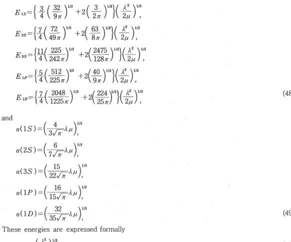
(8) A Linear Potential for Quark-Antiquark Pair System. 9^n,=N{ar)LZL,+w{a2rl)exp(-^a2r2)Y^(0.<p), (41) where n =L+p+l{the principle quantum number), a2=^&>=/^ and Z is a Laguerre polynomial. The normralization constant N is given by. ^(p+L+^)(p+L-^)-^-x^xp\' (42) A few of these functions which are denoted by the combination (n,L) are written down. V,s=(-^)wexp(-^a2r2) Y»(0,<p), 1/2 2 I 4a3 \"2. 'Plp=./^-. 3 \ /^. arexp(-^-a2r2)Yi(0. cp),. •3 \ 1/2 T/_4ff^v'2 a2rtexp{--^a\r2)Yz(0.v), 'I/lo=Vl5^ Tt I - r,. /2( 4ff3 y^s [(—^)w4-a2r2) exp( -yff2r2) Y«(Q, y),. '2S-V 3. V,s=^(-^)v\m- 5a^+a4rf)exp(-^a2r2)Y,(9,v). (43) We treat, for example, IS state (the ground state) accoding to the above procedure. A. straightforward calculation gives the approximated IS state energy E?fl"'ox=^(o+ <Vzs\Ar\9is>. (44). =^,,+-^. =~T(t)~r i — , A-. /?r'a. Minimizing this with respect to k yields. "^-'-n-.f. >"•. <45'. a=(/uk)w=(^±= A^V'3 C46) ' Jt I •. Substituting eqs. (45) and (46) into eq. (44), we obtain. —{^Mi-JW. —(^r(^A-)"^H(^nr^'. V2. 'Pis(0)=(^-A/^. (47). When we use the variational method to the other states in the same way, we can fix the corresponding optimum coupling constant k (a,co) for each state. We summarize the minimized energies and a values as follows,. (25).
(9) Masanobu HIRANO and Yoko IKEDA. 3_(^\13^(-^\13\(-^\13 Els=\~t{^7r) +2{~^) ]\'2n) ,. ^. E:. =iZ( TL\13 ^( 6^\. AV'3 2/u ),. __JUi^25_y'3 ,^2475y'3VA2 y'3. E3s={t[1^) +2[m^) \{~2n),. E-{i(-H.T 4\225;r/+2(€)"3}(i)1:3 .Qjt! \\2n), 1_ Ew={^. (48). |2 2048 y'3 (•22A^S\( _^_\w. 1225^, ~v"\~25^/ S\2fi/ ,. and. 1(3. a(ls)=(w^^r a(2S)=. 6. 7,^. •Afl. ff(3s)=(wT^ a(lP)=. 16 15. A/^ 1/3. a(lp)=(-3^r. (49). These energies are expressed formally. ,=(^'\. (50). EnL= [~^~] £nL. We compare this with the exact value of eq.(34) for L=0 state in Table 2, where IP and ID states are also listed. The approximation for the level energy is very good.. Table 2. The comparison of a,, with obtained e ,,L for the lowest levels.. Level. IS 2S 35. a,i. En L. 2.338. 2.345. 4.088. 4.075. 0.3. 5.521. 5.498. - 0.4. IP ID. rror7Q. 0.3. 3.368 4.254. For many purposes, the wave function at the origin is used. So its replacement by the. harmonic oscillator wave function is important. From eqs.(38) and (47) we find. w. (51). V&t'prox(0}/V^(0)=[-^} =0.92, Jt,. showing that the approximation is good to 8% even in zeroth order. We next present the expectation value <!/;'> , <l/r3> and/<r2>,. (26). calculated by the.
(10) A. Linear Potential for Quark-Antiquark Pair System. wave function of eq. eq. (43) (43) and and eq.(49). These were used in the previous papers10' or will be used function of in the; forthcoming paper. They are. ) =—f=a^ ls ) = { ~^Z2^. lf3. r '-- ^K~ "~ ' \ 'd7['"'~/,. <2S|^S>^2S)^(^)" <3s^i3s>=^ff(3s)=s(^r. <lp^lp>^^w l^n n,= 16 ..M n^_16^ 32 , y'3. 1tiu)>=-i57ra(12))=t^27^>,. ap^lp>-^lp^^ <lD\^lD>=^a(lDr=^, I r2HS w= J^- —l^=J3r(3/^-]-^3 i^'1-5 >= V? ^asT=VTI^—7/l7. In the last, we mention that the reason why this simple replacement of the linear potential by a harmonic oscillator potential works so well is easily understood. For large r, they behave. in the very different way, but the wave function falls off exponentially so that this region is of no importance. For small r, the boundary condition ^?(0)==0 in eq.(10) suppresses this region though the potentials are also different. Therefore, the region where the wave functions for both potentials behave rather similarly, contributes to the calculation of the expectation value.. References. 1) T.M. Yan, "Theoretical Charmonium Spectroscopy", Vth Internatioal Conference on Experimental Meson Spectroscopy, Boston, 1977. J. D. Jackson, "New Particle Spectroscopy", European Conference on Particle Physics, Budapest, July, 1977. K.Gottfried,"The Spectroscopy of The New Particle" 1977 International Symposium on Lepton and Photon Interaction," Hamburg, Angst, 1977. T. Appelquist, R,M. Barnett and K. Lane, SLAC-PUB-2100 (to be published in Annual Review of Nuclear and Partical Science, Vol. 28). J.D. Jackson, C. Quigg and J.L. Rosner. "New Particles, Theoretical;' Proceedings of The 19th International Conference on High Energy Physics, Tokyo, 1978. 2) K. Verkleman, "e+e- Reactions;' Proceedings of The 19th International Conference on High Energy Physics, Tokyo, August, 1978.. 3) H.D. Politzer, Physics Reports 14 (1974), 129. H.Fritzsch, Prep. Th.2483-CERN, 1978.. (27).
(11) Masanobu HIRANO and Yoko IKEDA. 4) E. Eichten et al., Phys. Rev. Letters 36 (1976), 500. B. J. Harrington, S.Y. Park and A. Yildiz, Phys. Rev. Letters 34 (1975), 168 ; Phys. Rev. Letters 34 (1975), 706.. J.S. Kang and H.J. Schnitzer, Phys. Rev. D12 (1975), 841 ; Phys. Rev. D12 (1975), 2791. 5) K. Wilson, Phys. Rev. D10 (1975), 2445. J. Kogut and L. Susskind, Phys. Rev. Dll (1975), 395.. 6) J.F. Willemsen, Proceedings of Summer Institute on Particle Physics, SLAC.July, 1974. Edited by M.C. Zipf. 7) A. Martin, Phys. Letters 67B (1977), 330 ; Phys. Letters 70B (1977), 192. H. Grosse, Phys. Letters 68B (1977), 343.. 8) T. Appelquist, M. Dine and I.J. Muzinich, Phys. Letters 69B (1977), 231. 9) H.J. Schnitzer, in Proceedings of Conferens on Experimental Meson Spectroscopy, Boston, April, 1977.. 10) M. Hirano and Y. Matsuda, Prog. Theo. Phys. 60 (1978), 1490; Prep. HUE-KTC 79210, February, 1979. 11) S. Flugge, Practical Quantum Mechanics (Springer-Verlag, 1974) p.101. W.Pauli.PW; Lectures on Physics, Vol. 5 (The MIT Press, 1977) p. 126.. 12) H. Hochstadt, The Functions of Mathematical Physics (John Wiley and Sons, 1971). 13) M. Abramwitz and J.A. Stegan, Handbook of Mathematical Functions (National Bureau of Standard, Washigton D.C. 1964).. 14) ^a^-, ^W\\m\, -<S <8;&^&^IH (S?ftl973) p.l88. 15) D. Gromes and 1.0. Stamatescu, Nucl. Phys. B122 (1976), 213.. H. Schnitzer, Phys. Rev. D13 (1975), 74; Phys. Rev. Letters 35 (1975), 1540.. (28).
(12)
図


関連したドキュメント
Theorem 4.8 shows that the addition of the nonlocal term to local diffusion pro- duces similar early pattern results when compared to the pure local case considered in [33].. Lemma
The first case is the Whitham equation, where numerical evidence points to the conclusion that the main bifurcation branch features three distinct points of interest, namely a
[18] , On nontrivial solutions of some homogeneous boundary value problems for the multidi- mensional hyperbolic Euler-Poisson-Darboux equation in an unbounded domain,
Kilbas; Conditions of the existence of a classical solution of a Cauchy type problem for the diffusion equation with the Riemann-Liouville partial derivative, Differential Equations,
Here we continue this line of research and study a quasistatic frictionless contact problem for an electro-viscoelastic material, in the framework of the MTCM, when the foundation
The study of the eigenvalue problem when the nonlinear term is placed in the equation, that is when one considers a quasilinear problem of the form −∆ p u = λ|u| p−2 u with
Then it follows immediately from a suitable version of “Hensel’s Lemma” [cf., e.g., the argument of [4], Lemma 2.1] that S may be obtained, as the notation suggests, as the m A
Classical Sturm oscillation theory states that the number of oscillations of the fundamental solutions of a regular Sturm-Liouville equation at energy E and over a (possibly
