The Role of Large-Scale Topography in the
Northern Hemisphere Annular Mode (Extended
Abstract)
著者
Yamazaki Koji, Ogasawara Atsushi, Nakazawa
Rui, Mukougawa Hitoshi
雑誌名
The science reports of the Tohoku University.
Fifth series, Tohoku geophysical journal
巻
36
号
4
ページ
510-513
発行年
2003-05
The Role of Large-Scale
Topography
in the Northern
Hemisphere Annular
Mode
(Extended Abstract)
KOJI YAMAZAKI"2, ATSUSHI OGASAWARA', RUI NAKAZAWA3 and HITOSHI MUKOUGAWA4
'International Arctic Research Center/FRSGC
'Graduate School of Environmental Earth , Science, Hokkaido University,
Sapporo, 060-0810
'Hewlett -Packard Japan, Ltd.
'Disaster Prevention Research Institute , Kyoto University (Received December 26, 2002)
1. Introduction
The leading mode of variability of the extratropical circulation called "Arctic Oscillation" (AO) or Northern Hemisphere annular mode, which is identified as the leading empirical orthogonal function (EOF) of sea level pressure (SLP) anomalies during cold season poleward of 20N, is characterized by annular structure and pressure dipole between Arctic and mid-latitudes (Thompson and Wallace, 1998, 2000).
There has been a debate whether the annular mode is a physical mode or an apparent mode (Deser, 2000, Ambaum et al., 2001, Wallace, 2000). The AO has two centers of action in mid-latitudes, i.e., one in Atlantic and the other in Pacific. However, there is no correlation between the Atlantic center and Pacific center (Deser, 2000). Ambaum et al., (2001) claims that AO is not a physical mode and the well-known North Atlantic Oscillation (NAO) is a physical mode.
For dynamics of annular mode, transient eddy and/or planetary wave coupling with large-scale topography is important in terms of interactions with mean zonal flows. In this study, we examine effects of large-scale topography on the annular mode using an atmospheric general circulation model (AGCM).
2. Experiments and analysis methods
The model used for this study is CCSR/NIES AGCM version 5.4. The resolution of the model is T21 in horizontal and 24 levels in vertical (top level 1 hPa). The experi-ments run under a perpetual January condition and climatological SSTs. The data for 7300 days after the spin-up period is used for analysis.
Four experiments are done with and without North American orography and Eurasian orography as f011ows : "Control run" (standard topography), "Himalaya run" (only Eurasian mountains), "Rockies run" (only North American mountains), and "No
511
mountain run" (no mountains).
The analysis in this study is based on 243 30-day mean fields . As analysis methods, we use EOF analysis and teleconnectivity analysis. We calculate EOFs based on three domains : Northern Hemisphere (poleward of 20°N), Atlantic sector (90°E-22 .5°E) and Pacific sector (I12.5°E-112.5°E).
3. Results
All experiments show an AO-like variation pattern as the 1st EOF of the 30-day mean SLP of the Northern Hemisphere (Fig. 1). In Control run and Himalaya run, there are centers of action of AO-like pattern in Atlantic and Pacific . In Rockies run there is only one center in Atlantic, and in No mountain run there is no centers of action . Explained variance by EOF-1 is the largest in Himalaya run (45.5%) and the smallest in No mountain run (28.8%). Zonal-mean zonal wind regressed on EOF-1 is calculated (figures not shown). In Control run and Himalaya run, the spatial patterns are similar to that in the actual AO.
EOF-1s of 30-day mean SLP based on Atlantic sector and Pacific sector are
e o f — 1 control—run 38.2% clp no—mountain
5i
28.8% 7I :
*a a -10 i -00 -30 -40 -eo -ea -1a -40 -*0 -100 .110 50 0 40 30 20 10 0 -10 -30 -40 -00 -00 -40 -40 -so ,10 Himolc Rockies5i
31.9% 5IFS
40 30 30 a --40 -30 -40 -00 -40 -100 -110 ea 30 30 10 a -f13 -30 -40 -SO -00 -40 -S0 -100 -110Fig. 1. The first EOF of 30-day mean SLP field for the region poleward of 20N for
each run. The plotted values are regressions on PC-1 and converted to
control—run no—mountain -030 -0.3 -0.33 -045 -0.55 -0.6 -005 -0,7 -0,73 -0.25 -0.3 -0.33 -4.45 -0.55 -4.0 -4.7 -0.75 Rockies ra -03 -0.35 -0.45 -0.55 -0.4 -0,65 -0.7 -0.73 -0.3 -0.31 -0,45 -5.55 -0.1 -005 -0.7 -0.75
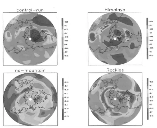
Fig. 2. Teleconnectivity map of SLP for each run. Plotted values are the minimum correlation coefficients.
examined (figures not shown). In Control run and Himalaya run, EOF-ls based on both sectors are AO-like pattern. In No mountain run, EOF-ls based on both sectors are annular, but that on Pacific sector does not show an action center in Atlantic. In Rockies run, E0E-1 based on Pacific sector is different from the annular mode.
Figure 2 shows teleconnectivity maps of SLP field that plot the strongest negative correlation coefficient. Even without mountains, the NAO-like teleconnection exists in Atlantic. The Eurasian and North American orography intensify the NAO-like varia-tion in Atlantic. Both mountains play roles in the NAO-like variation constructively. While over the Pacific, the Eurasian orography intensify the variation between East Siberia and Pacific, and the North American orography intensify the variation between Arctic and East Asia. Two mountains seem to play roles in variations in Pacific destructively.
Having examined one-point correlation maps on each centers of teleconnectivity, we find that NAO-like variation in Control, Himalaya and Rockies runs and the variation between Arctic and East Asia in Control run seem to associate with EOF-1 which likes the AO.
513
4. Summary and discussion
In EOF analysis, the Eurasian topography intensify AO-like variation pattern
remarkably in both the Atlantic and the Pacific sectors. While the North American
topography, in EOF analysis, intensify AO-like variation pattern in the Atlantic and, in
teleconnectivity analysis, raise teleconnectivity between the Arctic and East Asia which
seems to associate with the AO. Therefore, it seems that the each role of Eurasian
topography and North American topography in the Northern Hemisphere annular
mode is important in both the Atlantic and Pacific.
In general, Himalaya run shows similar variability with Control run. This is
probably because that the mean flows are similar, while those of Rockies run and No
mountain run are different from that in Control run. For instance, Icelandic low and
Aleutian low are realistically simulated in Control and Himalaya runs, while the other
two runs show poor simulations of these lows.
One puzzling aspect in the simulation is the annular mode in Control run is more
robust than observations and even EOF-1 on Pacific sector shows AO-like pattern. We
need to clarify the cause.
References
Ambaum, M.H.P., B.J. Hoskins, and D.B. Stephenson, 2001 : Arctic Oscillation or North Atlantic Oscillation ? J. Climate, 14, 3495-3507.
Deser, C., 2000 : On the teleconnectivity of the "Arctic Oscillation", Geophys. Res. Lett., 27, 779-782. Thompson, D.W.J., and J.M. Wallace, 1998 : The Arctic Oscillation signature in the wintertime
geopotential height and temperature fields, Geophys. Res. Lett., 25, 1297-2000.
Thompson, D.W.J., and J.M. Wallace, 2000 : Annular modes in the extratropical circulation. Part
I : Month-to-month variability. J. Climate, 13, 1000-1016.
Wallace, J.M., 2000 : North Atlantic Oscillation/annular mode : Two paradigms-one phenomenon,
Quart. J. Roy. Meteor. Soc., 126, 791-805.