西 南 交 通 大 学 学 报
第 56 卷 第 2 期
2021 年 4 月
JOURNAL OF SOUTHWEST JIAOTONG UNIVERSITY
Vol. 56 No. 2
Apr. 2021
ISSN: 0258-2724 DOI:10.35741/issn.0258-2724.56.2.33
Research articleEconomics
T
HE
S
OURCE OF
O
UTPUT
G
ROWTH
:
P
RODUCTIVITY
P
ERFORMANCE
IN THE
I
NDONESIAN
C
RUDE
P
ALM
O
IL
I
NDUSTRY
产出增长的来源:印度尼西亚原油棕榈油行业的生产力表现
Dyah Wulan Sari a,*, Haura Azzahra Tarbiyah Islamiya a, Wenny Restikasari a, Emi Salmah ba Department of Economics, Airlangga University, Surabaya, Indonesia,
*Coressponding author, dyаh-wulаnsari@fеb.unair.ac.id, wеnny.restikа[email protected], hаura.islа[email protected]
b Department of Economics, Mataram University, Mataram, Indonesia,
еmisalmа[email protected]
Received: January 16, 2021 ▪ Review: March 9, 2021 ▪ Accepted: April 5, 2021 ▪ Published: April 30, 2021
This article is an open-access article distributed under the terms and conditions of the Creative Commons Attribution License (http://creativecommons.org/licenses/by/4.0)
Abstract
Indonesia has become the largest producer and exporter of crude palm oil commodities in the world. Therefore, the production of CPO turns out to be very greedy for land. There are any problems in production CPO, therefore the study aims to develop a conceptual framework of the source of output growth, whether driven by input or productivity growth, and to implement this concept by investigating the source of output growth in the crude palm oil industry in Indonesia. The investigation applies firm-level panel data and follows a quantitative approach using general method of moments to estimate the production coefficients and calculate the input and productivity growth. The result shows that the output growth of the crude palm oil industry does not lead in productivity growth driven. It seems to be driven by input growth, not by productivity growth. Since growth is still driven by input, the crude palm oil industry will be less competitive in the world market. The high world demand for crude palm oil commodities from Indonesia must be met by using more efficient input factors, optimizing production scale, and supporting technological progress. The government, therefore, must have strategies that are more competitive in the global market.
Keywords:Source of Output Growth, Productivity Growth Driven, Crude Palm Oil
摘要 印度尼西亚已成为世界上最大的棕榈油商品生产国和出口国。因此,首席财务官的生产对土
地非常贪婪。生产首席财务官中存在任何问题,因此,本研究旨在建立一个由投入或生产率增长 驱动的产出增长来源的概念框架,并通过调查原油棕榈油行业的产出增长来源来实施这一概念。
在印度尼西亚。该调查采用公司层面的面板数据,并采用一种定量方法,该方法采用一般的矩量 法来估算生产系数并计算投入和生产率的增长。结果表明,原油棕榈油行业的产量增长并未导致 生产力的增长。它似乎是由投入增长驱动的,而不是生产力的增长。由于增长仍受投入驱动,因 此粗棕榈油行业在世界市场上的竞争力将下降。必须通过使用更有效的输入因素,优化生产规模 并支持技术进步来满足印尼对世界上对棕榈油商品的高需求。因此,政府必须制定在全球市场上 更具竞争力的战略。 关键词: 产出增长的来源,生产力增长的驱动力,粗棕榈油
I. I
NTRODUCTIONIndonesia has become the largest producer and exporter of crude palm oil (CPO) commodities in the world, accounting for around 58.31 percent of total global CPO production. The world's need for CPO is triggered not only by food commodities but also by its use as a renewable energy source to replace fossil fuels. In this regard, CPO as a superior commodity plays an important role in providing an alternative energy source and contributing to economic development [1], [2].
Huge demand for CPO in the world encourages producers to raise their production, which increases the demand for material input, such as palm oil. The expansions of CPO production have had impacts on labor absorption as well as oil palm plantations; however, the development of these plantations has reduced and destroyed natural forest areas in Indonesia. CPO production has caused millions of hectares of conversion rainforest areas to abandoned lands in the form of shrubs and new critical lands [4], [5]. Lands are declared as abandoned when there is an inappropriate use of land, and critical lands are lands that have suffered damage causing the loss or reduction in function. The expansion of land for oil palm cultivation means that tropical rainforests with high carbon stores have to compete with the most profitable alternative land uses. In 2014, the ratio of oil palm production to the total area of oil palm plantations in Indonesian CPO production was only 3.73 tons/ha from plantations covering 10.96 million hectares, lower than the same ratio in Malaysia, which was 4.82 tons/ha from plantations covering 4.5 million hectares. Data from the Indonesian Ministry of Agriculture shows that, in 2015, the area covered by oil palm plantations reached 11.26 million hectares, and in 2017, it increased to 14.05 million hectares. Furthermore, in 2019, the area of oil palm plantations was about 14.68 million hectares, and also in 2020 the area of palm plantations increased to 2.3 percent or around 15.02 million hectares [2], [3].
The Indonesian government’s efforts to increase CPO production have received positive responses from both local and foreign investors. An appropriate government policy is still needed, however, to support this development of the CPO industry, making it more competitive in the global market and sustaining its growth. The high-growth performance in the CPO industry raises the question of whether an increase in world demand for CPO commodities can also preserve and sustain Indonesia's natural forest areas. To assess this issue, it is crucial to examine the source of output growth of the CPO industry in Indonesia. The increased production in the CPO industry can be driven by rapid growth in input factors or by improvement in productivity. To increase production, a firm can either use more input factors or use the same number of inputs more efficiently (e.g., using more efficient techniques and scales, using more advanced technology). The growth rate of productivity is a useful indicator of the source of output growth, which can then be used to measure the change in productivity over time. By using the same number of input factors—especially oil palm material inputs—to increase its output, a firm can preserve Indonesia’s natural forests. This study, therefore, will investigate the source of output growth in the CPO industry.
II. L
ITERATURER
EVIEW A. The Source of Output GrowthThis study starts to develop a conceptual framework of the source of output growth from a basic production function. A production function is a convenient way of describing the productive capabilities of a firm. It specifies a relationship between the quantities of productive factors (e.g., labor, machinery, fixed assets, raw material, energy used, and the amount of product attained). The production function expresses the amount of product that can be produced from every combination of input factors, assuming technology used is a constant. Based on
economic principles, a firm will maximize its production using a given input or will minimize the use of input to produce a given output [6], [7].
There are two types of sources of output growth: input-growth-driven and
productivity-growth-driven. This study will modify the
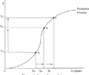
concept of input growth driven or productivity growth driven, which was introduced by [8], [9], [10], [11], [12], [13]. A firm can achieve rapid output growth by simply using more factors of production. Alternatively, rapid output growth can also be achieved by using the same number of inputs more productively (e.g., by using a better technique and scale of production or upgrading its technology). These options inspire economists to differentiate between input growth driven and productivity growth driven processes. In processes that are input growth-driven, an increase in production can be sourced by using more input factors. Firms can increase production by increasing worker overtime, hiring more workers, and operating their plants with a lot of machinery. However, for simplicity, we assume that firms here produce a single output (Y) with a single input factor (X) only. It also assumes that the most efficient available production methods are applied with a given state of engineering technical knowledge. The production frontier can be drawn, such as in Figure 1. At point A, a firm produces output YA using input XA. If the firm
wants to upsurge its production, it can increase its input to XB or XC. Then, the firm can obtain the
output of YB or YC. When a firm wants to raise
its output from point A to point B or point C, it will deal with more input factors. In this case, a firm always strives to produce efficiently. In other words, a firm always attempts to produce the maximum level of output for a given dose of inputs. Since firms involve with more and more input factors, then firms can produce more and more output. This is recognized as the source of output growth through input factor driven.
Figure 1. Input factor driven
In contrast, to increase firms' production, producers can provide engagement with the same number of inputs but increasing their productivity. The productivity growth driven can be transmitted through three channels: using more efficient factor input, optimizing production scale, and changing to advantage technology. The source of growth because of these three channels is acknowledged as total factor productivity (TFP) growth driven rather than productivity growth driven. However, in this study, we are referring to use the term "productivity-growth-driven".
Figure 2. Efficiency driven
In reality, some producers may produce their output using their inputs less efficiently. This allows the location of the firms beneath their production frontier. In Figure 2, firm N operates inside its production possibility frontier. To produce output YN, firm N employs input XN,
operating inefficiently. The same output could be produced with fewer inputs. At point L, obtaining output YN only needs input XL. In this situation,
firm N can move up to the frontier at point M, using the same input XN, it obtains YM. Since
firms use the same amount of input and then produce more output, this source of output growth is called efficiency driven.
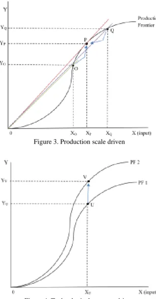
Figure 3. Production scale driven
Figure 4. Technological progress driven
Moreover, the source of growth can be driven by optimizing the scale of production. The simple way to measure productivity is just the ratio between output and input, Y/X. The productivity at point P (YP/XP) is greater than the productivity
at point O (YO/XO) or point Q ((YQ/XQ). When
drawing the line from 0 (the original point), the slope of the line at point P is greater than at point O and point Q. Therefore, any firm will have maximum productivity when its production moves from point O to point P or from point Q to point P. This source of output growth is called production scale driven.
Finally, the source of output growth can be driven by technological progress. At point U, a firm yield output YU using input XU. When there
is technological change, a firm can shift its production from point U to point V. At point V, a firm produces a greater output (YV) with the
same amount of input (X1). This technology
progress causes the production frontier to move up from PF1 to PF2. This source of growth is
known as technological progress.
B. Productivity Measurement
Measuring the growth rate of output can be based on production theory. The production function can be expressed by:
𝑌 = 𝑓(𝑋, 𝛽) (1) where 𝑌 symbolizes output, 𝑋 represents the vector of input factors, and в denotes vectors of parameters to be estimated. This study will apply the simplest Cobb-Douglas form. This function assumes that elasticity of substitution between inputs is unitary [14], [15], [16]. Implementing the Cobb-Douglas production function, the equation (1) can be specified as follows:
𝑌 = 𝐴𝐾в1𝐿в2𝑀в3𝐸в4 (2a)
Equation (2a) can be converted into a natural logarithm form such as:
𝑙𝑛𝑌 = 𝑙𝑛𝐴 + в1𝑙𝑛𝐾 + в2𝑙𝑛𝐿 + в3𝑙𝑛𝑀 +в4𝑙 (2b) where 𝑌 is the output to be produced. 𝐾, 𝐿, 𝑀, and 𝐸 represent respectively capital stock, labor input, raw material and fuel, gas and electricity. All of these are used in the production process as input factors. A is identified as technology.
The equation (2b) describes the Cobb-Douglas production function with assuming a variable return to scale. The return to scale could be increasing, decreasing, or constant [17]. If we add all the estimated coefficients (в1+ в2+ в3+
в4) and the summation is greater (less) than one, the production function will exhibit increasing (decreasing) returns to scale. If it equals to one, the production function shows a constant return to scale. This implies that if all of the inputs are doubled, the output will be exactly double. However, when summating of estimated coefficients is greater (less) than one, the production function exhibits increasing (decreasing) returns to scale. This indicates that if all of the inputs are doubled, the output will be more (less) than double.
Furthermore, to calculate the productivity growth, we take the first derivative from equation (2b) for 𝑡, it will give:
𝜕𝑙𝑛𝑌 𝜕𝑡 = 𝜕𝑙𝑛𝐴 𝜕𝑡 + в1 𝜕𝑙𝑛𝐾 𝜕𝑡 + в2 𝜕𝑙𝑛𝐿 𝜕𝑡 +в3 𝜕𝑙𝑛𝑀 𝜕𝑡 + в4 𝜕𝑙𝑛𝐸 𝜕𝑡 (3a) 1 𝑦 𝜕𝑌 𝜕𝑡 = 1 𝐴 𝜕𝐴 𝜕𝑡+ в1 1 𝐾 𝜕𝐾 𝜕𝑡+ в2 1 𝐿 𝜕𝑙𝑛𝐿 𝜕𝑡 +в3 1 𝑀 𝜕𝑀 𝜕𝑡 + в4 1 𝐸 𝜕𝐸 𝜕𝑡 (3b) 𝑌̇ 𝑌= 𝐴̇ 𝐴+ в1 𝐾̇ 𝐾+ в2 𝐿̇ 𝐿+ в3 𝑀̇ 𝑀+ в4 𝐸̇ 𝐸 (3c)
𝐴̇ 𝐴= 𝑌̇ 𝑌− [в1 𝐾̇ 𝐾+ в2 𝐿̇ 𝐿+ в3 𝑀̇ 𝑀+ в4 𝐸̇ 𝐸+ в5] (3d) where 𝐴̇
𝐴 is the productivity growth, and 𝑌̇ 𝑌 is the output growth. The input growth contains capital growth (в1 𝐾̇ 𝐾) , labor growth (в2 𝐿̇ 𝐿) , input material growth (в3 𝑀̇
𝑀) and energy growth (в4 𝐸̇ 𝐸). However, the productivity growth 𝐴̇
𝐴 in this calculation only captures technical efficiency growth.
For optimizing the scale of production, the production function should be assumed a constant return to scale. When the production function is a constant return scale, productivity will be at its highest. Hence, we rearrange equation (2a) into equation (3b).
в1+ в2+ в3+ в4=1, в2 = 1 − в1− в3− в4 (3a) 𝑌 = 𝐴𝐾в1𝐿1− в1− в3 − в4𝑀в3𝐸в4 (3b)
Then, equation (3b) can be converted into a logarithm natural form such as:
𝑙𝑛𝑌 = 𝑙𝑛𝐴 + в1𝑙𝑛𝐾 + (1 − в1- в3-в4)𝑙𝑛𝐿 +в3𝑙𝑛𝑀 + в4𝑙𝑛𝐸 (4a) 𝑙𝑛𝑌 − ln 𝐿 = 𝑙𝑛𝐴 + в1(𝑙𝑛𝐾 − 𝑙𝑛𝐿) +в3(𝑙𝑛𝑀 − 𝑙𝑛𝐿) + в4(𝑙𝑛𝐸 − 𝐿𝑛𝐿)(4b) 𝑙𝑛𝑌 𝐿= 𝑙𝑛𝐴 + в1𝑙𝑛 𝐾 𝐿+ в3𝑙𝑛 𝑀 𝐿+ в4𝑙𝑛 𝐸 𝐿 (4c) ln𝑦 = 𝑙𝑛𝐴 + в1𝑙𝑛𝑘 + в3𝑙𝑛𝑚 + в4𝑙𝑛𝑒 (4d) Besides that, a time trend variable will also be included to identify any trend in the data. It could be interpreted as technological change. Therefore, to capture the impacts of any potential technological changes on the output level of an industry, the equations (2b) and (4d) are augmented with a time trend. It could be expressed as follows:
𝑙𝑛𝑦 = 𝑙𝑛𝐴 + в1𝑙𝑛𝑘 + в2𝑙𝑛𝐿 + в3𝑙𝑛𝑚 + в4𝑙𝑛𝑒 + в5𝑡 (5a)
𝑙𝑛𝑦 = 𝑙𝑛𝐴∗+ в1𝑙𝑛𝑘 + в3𝑙𝑛𝑚 + â4𝑙𝑛𝑒 +в5𝑡 (5b) where 𝑡 is a time trend variable that indicates any potential technology changes in the industry. Equation (5a) shows a production function assuming a variable return to scale (VRS), while equation (5b) assuming a constant return to scale (VRS). Finally, to estimate the growth rate of productivity, which captures technical efficiency, optimal scale, and technological progress, we will use the estimated coefficients from equation
(5b). Hence, the formulation can be written formally as follows: (𝐴̇ 𝐴) ∗ =𝑌̇ 𝑌− [в1 𝐾̇ 𝐾+ (1 − в1− в3− в4) 𝐿̇ 𝐿+ в3 𝑀̇ 𝑀+ в4 𝐸̇ 𝐸+ в5] (6) where 1 − в1− в3− в4 equals to в2. A firm can achieve rapid output growth by simply using a more conceivable set of inputs known as input growth driven. Alternatively, rapid output growth can also be achieved using the same amount of inputs more productively, which is recognized as productivity growth driven. From the equation (6), input growth driven is the summation of the growth of capital, labor, raw material and energy weighted by share input factor coefficients (в1 𝐾̇ 𝐾+ (1 − в1− в3− в4) 𝐿̇ 𝐿+ в3 𝑀̇ 𝑀+ в4 𝐸̇ 𝐸+ в5), while total factor productivity growth driven, which considers technical efficiency, optimal scale, and technological progress, can be revealed by (𝐴̇ 𝐴) ∗ .
III. M
ETHODS A. Data SourcesThis study will use the data on the CPO manufacturing industry to apply the conceptual framework of the source of output growth, whether driven by input factors growth or productivity growth. The data are obtained from an annual survey of medium and large manufacturing establishments conducted by the Indonesian Central Board of Statistics (BPS), covering the selected period from 2010 to 2014. The survey will involve all manufacturing enterprises which employ at least 20 workers each every year. Large manufacturing enterprises involve more than 99 workers, while medium manufacturing enterprises engage with 20 to 99 workers.
This study utilizes unbalanced panel data for a crude palm oil (CPO) industry. This industry includes processing palm oil into crude oil, which must be further processed, and this product is usually used by other industries. The CPO industry in international standard industrial classification (ISIC) at the 5-digit level is coded with 10431. The annual observations of the CPO industry vary from 411 firms in 2010, 472 firms in 2011, 478 firms in 2012, 548 firms in 2013, and 598 firms in 2014. The total number of observations during the period of 2010 to 2014 is 2,607 firms. This is because lag variables are included in the model, so the number of observations is reduced to 1,848 firms. A
balanced panel dataset is constructed when calculating the growth. After the adjustment process for making a balance panel data, the number of observations becomes 377 each year.
The variables for each firm consist of output, capital stock, labor, raw materials, and energy. The output variable is proxy by the gross output. Gross output refers to the total output produced by a firm in a given year. The capital stock is estimated all value of fixed capital purchase, addition and construction, major repair, sales, or reduction of fixed capital as well as the depreciation of fixed capital during a given year. The fixed capital can be distinguished from land, buildings, machinery, equipment, and vehicles. However, capital stock data are subject to numerous missing values from year to year [18], [19], [20], [21]. The capital series are regressed against once lagged real output values to estimate capital at establishment level. The estimations are then imputed for establishments which missing values.
Based on the production function concept discussed above, all variables should be measured in physical units that are equivalent across firms. Labor input can be measured by the number of workers or man-hours. Because the data on man-hours are not available, labor input
will be measured using the number of workers. However, the output and material input, energy, and capital stock are measured in monetary terms and valued in million rupiah. Raw material is the total cost of domestic and imported raw material used in the production process, while energy is the total expenditure on gasoline, diesel fuel, kerosene, public gas, lubricant, and electricity. When an output or input is valued in monetary terms, a few things must be considered to implement the above technique. All the data on the monetary values will be deflated into real values or constant prices in 2010 using the wholesale price index. Since all variables in monetary terms are deflated as constant prices, this measurement is equivalent to physical units. Therefore, this study also needs other supplementary data such as the wholesale price index. These data are published by BPS and are applied to deflate the monetary value outputs and all inputs into real values or at constant prices in 2010. All variables of output and input factors are expressed in the form of logarithm natural and deviation from their geometric sample means and summarized in Table 1. Suppose the geometric mean of 𝑌 is 𝑌̅, the transformed variable of 𝑌 will be 𝑦 = 𝑙𝑛𝑌 − 𝑙𝑛𝑌̅.
Table 1.
A statistical summary of variables
Variables Unit Obs Mean SD Min Max
𝑦 (output) ln (million rupiahs) 2,507 0.0000 0.9910 -4.8460 4.4340
𝑦/𝑙 (output per labor) ln (million rupiah per worker) 2,507 0.0000 0.8977 -4.8751 3.9944
𝑘 (capital) ln (million rupiah) 2,507 0.0000 1.5026 -5.4900 7.7630
𝑘/𝑙 (capital stock per labor) ln (million rupiah per worker) 2,507 0.0000 1.4165 -5.2007 6.3861
𝑙 (labor) ln (worker) 2,507 0.0000 0.8743 -2.1300 4.3330
𝑚 (raw material) ln (million rupiah) 2,507 0.0000 1.1110 -5.8020 4.7980
𝑚/𝑙 (material per labor) ln (million rupiah per worker) 2,507 0.0000 1.0919 -5.8525 4.5385
𝑒 (energy) ln (million rupiah) 2,507 0.0000 1.1694 -5.4770 4.8100
𝑒/𝑙 (energy ln (million rupiah per worker) 2,507 0.0000 1.0919 -5.8525 4.5385
𝑡 (time trend) time 2,507 0.2320 1.8381 -2.5000 2.5000
Note: ln = logarithm natural; Obs = Observation; SD = Standard Deviation; Min = Minimum; Max = Maximum
B. Short Dynamic Panel Data Regression
To estimate equation (5), we need to deal with panel data with a large number of cross sections and a small number of time periods. Hence, the econometric equation of the panel data can be expressed as follows:
𝑦𝑖𝑡 = ρ𝑦𝑦𝑖𝑡−1+ б𝑛𝑥𝑛𝑖𝑡+ е𝑖𝑡, (7a)
е𝑖𝑡 = щ𝑖+ 𝑢𝑖𝑡 (7b) where yit is an endogenous variable and 𝑦𝑖𝑡−1 is a lag value of the endogenous variable. 𝒙𝒊𝒕 is a column vector of 𝑛 regressors. б′s are vectors of parameters to be estimated and subscript 𝑖 and 𝑡
represent the individual firm and period. е𝑖𝑡 is the error term, consisting of the unobserved individual-specific effects ( щ𝑖) and the observation-specific errors (𝑢𝑖𝑡).
Several problems may be embedded in е𝑖𝑡 when estimating Equation (7a), leading to simultaneous or serial correlation of residuals across observations within firms. For example, if the variation in 𝒙𝒊𝒕 is assumed to be exogenous to 𝑦𝑖𝑡 the estimation will be biased when this condition is not met, leading to endogeneity bias. To overcome this issue, a difference GMM estimation has been introduced [22]. When this
strategy is adopted, all regressor variables are transformed, usually by applying first differentials, whereby lagged levels of the dependent variable serve as instruments, and the lagged levels of regressors are adopted as instruments for the first-differenced regressors. However, if the behavior of the dependent variable is represented by a random walk, the autoregressive estimator tends to be downward biased, in finite samples in particular. Therefore, lagged regressor levels are weak instruments for the first-differenced regressors [23].
The dependent variable can be stationary or stationary. If the dependent variable is non-stationary, the dependent variable's behavior can be said as a random walk.
The problem mentioned above might be overcome by using the original equation in levels to obtain a system of two equations, representing the first differences and levels equations, respectively, resulting in a system GMM [24]. The original equation (equation (7a): 𝑦𝑖𝑡 = ρ𝑦𝑦𝑖𝑡−1+ б𝑛𝑥𝑛𝑖𝑡+ е𝑖𝑡) is in level. However, there is a problem when we use the lagged variable as an instrument. It is a weak instrument and causes the estimator to tend to be downward biased, in finite samples in particular. For overcoming the problem, the original equation is transformed to a first different equation (∆𝑦𝑖𝑡 = ρ𝑦∆𝑦𝑖𝑡−1+ б𝑛∆𝑥𝑛𝑖𝑡+ ∆е𝑖𝑡). Then, we can get instruments from both first differences and level equations. This system of two equations is called a system GMM. In this system of equations, additional instruments can be obtained to increase efficiency. Moreover, the variables in levels will be instrumented with suitable lags of their first differences. However, the first differences should not be correlated with the unobserved individual effects [25].
An alternative approach to get instruments is replacing first differencing with forward orthogonal deviations transformation [24]. It is because the transformation does not feature the lagged variables. If an individual fixed effects problem arises, we can eliminate this problem using forward orthogonal deviations transformation. Furthermore, the GMM model can be applied with one-step or two-step estimations [26]. Although the two-step estimation is better suited for estimating the coefficients and is asymptotically more efficient, the standard errors tend to be downward biased. This issue can be rectified by applying finite-sample correction to the two-step covariance matrix, rendering the process more efficient [27].
When applying the GMM method to estimate Equation (7), it is needed second-order autocorrelation AR(2) test, and the validity of system GMM should also be performed.
In the GMM estimation procedure, two types of statistic tests should be performed. Those are the Arellano-Bond AB test and Sargan/Hansen test [28]. The AB test is a statistic test for first-order autocorrelation AR (1) and second-first-order autocorrelation AR (2). Under the assumption that no second-order serial correlation of the error term exists, the first-difference equation produces unbiased and consistent estimators. The test for AR(1) process in first differences usually rejects the null hypothesis, whereas the test for AR(2) will detect autocorrelation in levels. The Sargan/Hansen test is a statistic test for the validity of instruments used in the GMM estimation procedure. Moreover, a validity test should be conducted to ascertain if the condition of the over-identifying restriction has been met. This condition means that instruments used in the GMM estimation procedure are enough or valid. Sargan test [29] can be employed for this purpose, as it is based on the assumption that the model parameters are identified through a priori restrictions. The Sargant test is using a chi-squared (𝜒2) distribution with df = m-k, where m is the number of instruments and k is the number of endogenous variables. The null hypothesis is valid for over-identifying restrictions. If the null hypothesis is rejected, this condition means that the GMM estimation procedure instruments are not enough or valid. Moreover, as the value of Sargan statistic is inconsistent when nonsphericity arises in the errors, the Hansen J test can also be implemented to test for the over-identification restriction with the same null hypothesis [30]. In this case, these tests are equivalent. Furthermore, a difference in Hansen test is performed to test the validity of subsets of instruments. It offers automatic testing for the validity of instrument subsets, support for observation weights, and the forward orthogonal deviations transform. If one performs estimation with and without a subset of suspect instruments, under the null of joint validity of the full instrument set. The regression without the suspect instruments is called unrestricted regression because it imposes fewer moment conditions. The difference in the Hansen test will be possible if the unrestricted regression has sufficient instruments to be identified. The difference in Hansen test statistics is itself asymptotically χ2, with the degrees of freedom
The difference or system generalized method of moments (GMM) estimators can be implemented in the study. Both are general estimators designed for situations with few periods and many individuals, independent variables that are not strictly exogenous or may have fixed effects, heteroskedasticity, and autocorrelation within individuals [30]. This study will select one of them with the most suitable one for estimating equations (7a) and (7b).
IV. R
ESULT ANDD
ISCUSSIONThe coefficients of both Cobb Douglas production functions in equations (5a) and (5b) are appropriate to be estimated using system GMM. All statistical tests of autocorrelations, validity for over-identifying restrictions, and the validity of subsets of instruments support that both equations are assessed with the system GMM procedure. We estimate the coefficients of both Cobb-Douglas production functions, assuming a variable return to scale (VRS) and another assuming constant return to scale (CRS). The estimation coefficients results of both Cobb Douglas production functions are reported in Table 2.
The pattern of serial correlation in the first-differenced residuals is consistent with the assumption that the 𝑢𝑖𝑡 disturbances are serially uncorrelated so that ∆𝑢𝑖𝑡 should have significant first-order serial correlation but no significant second-order serial correlation. These are revealed by the significant coefficients of the lagged dependent variable (𝑦𝑖𝑡−1) at the level of significances = 1 % on both VRS and CRS models (Table 2). Furthermore, the statistic test
for AR (1) for both production functions has a significant first-order serial correlation. However, the statistic test for AR (2) shows that we do not reject the null hypothesis of no autocorrelation at any significant level. This indicates that there is no second-order serial correlation in the models. This evidence means that the AR (1) on both production functions are well specified for the data series used in this study.
For assessing the validity of the over-identifying restrictions, a Sargan test is implemented. In Table 2, the Sargant statistic value reports the p-values for the null hypothesis of the validity of the over-identifying restrictions. We do not reject the null hypothesis in all specifications models of VRS and CRS production functions at any significance levels. Moreover, the difference-in-Hansen value indicates the p-values for the validity of the additional moment restriction, and we also do not reject the null hypothesis at any significance level, meaning the additional moment conditions are valid in both models.
The estimated coefficients of both production functions are statistically different from zero at the significance level of = 1 %, except for a labor coefficient in the CRS model at the significance level of = 5 %. Additionally, all coefficients have positive signs as expected, except for the coefficient of time trend variable (t). It has a negative sign on both VRS and CRS models. The estimated coefficients of input variables can be interpreted as output elasticity for each input factor. This elasticity determines how much the percentage change in output when the input factor increases by one percentage change.
Table 2.
The estimated coefficients of Cobb-Douglass production function
Variables VRS Model CRS Model
Coefficients Coefficients Constant 0.0467*** 0.0354*** (0.0086) (0.0086) 0.2507*** (0.0677) 𝑦/𝑙𝑡−1 0.1966*** (0.0699) k 0.0810*** (0.0043) k/l 0.0905*** (0.0057) l 0.0344** (0.0193) m 0.4575*** (0.0142) m/l 0.5042*** (0.0102) e 0.1909***
(0.0098) e/l 0.2128*** (0.0087) t -0.0669*** -0.0610*** (0.0076) (0.0081) AR (1) [0.0000] [0.0000] AR (2) [0.3870] [0.3990]
Sargan test of over-identifying restrictions [0.2710] [0.7260] The difference in the Sargan test (null H = exogenous) [0.1610] [0.5230]
Number of Observation 1848 1848
Number of firms 556 556
Number of instrument 10 9
Note: The symbols of *** and ** indicate statistical significance at the = 1% and = 5% levels.
The symbols of ( ) and [ ] are standard error and probability value, respectively
The VRS model in Table 2 shows that the estimated coefficient of capital (0.0810) is greater than the estimated coefficient of labor (0.0344). This exhibits that the CPO manufacturing industry is more capital intensive than labor intensive. This industry absorbs less labor and requires a larger amount of investment to purchase. This industry uses a large percentage of its capital to buy expensive machines, compared to their labor costs, and thus has a high percentage of fixed assets, such as properties, plants, and equipment. As a result, capital-intensive industries require a high volume of production to be able to provide an adequate return on investment. This also indicates that small changes in sales can lead to big changes in profits and return on invested capital.
The estimated coefficients of raw material (0.4575) and energy (0.1909) are greater than the estimated coefficients of capital and labor. In economics, this shows that the value added is very small and the production cost is very large. The value added is the revenue received by the owners of the capital and workforce. The revenue received by the capital owner is known as profit and the revenue received by the workforce is called wage or salary. The production cost in this case is the expenditures to buy raw materials and energy. Thus, the value added is the difference between the sale price and the production cost for raw materials and energy.
When we add up all the output elasticity with respect to its input, the total elasticity of output is less than one. The total coefficient of input factors will be 0.7638 (0.0810 + 0.0344 + 0.4575 + 0.4575). This shows that the total elasticity of output of the VRS model exhibits diminishing returns when scaled, meaning if we double the input, the output will increase by less than double. A proportionate increase in the input does not lead to an equivalent increase in output; the output increases at a declining rate. The law of
diminishing returns is supposed to operate, resulting in higher average cost per unit.
Using the estimated coefficients of the VRS model, the growth rate of input and output factors and total factor productivity will be constructed for the CPO industry in each year with a constant price of 2010. The calculation of the source of output growth will be also classified into ownership. The results are presented in Tables 3, 4, and 5, respectively. To investigate the source of growth, it is necessary to look at the growth rates of input and output factors and TFP. During the observed period, most of the output of the CPO industry grew positively. However, the average annual growth of output for all samples tended to decline from 87.41% in 2011 to 5.09% in 2014. The average annual growth of output for foreign and domestic firms also tended to decrease from 92.07% in 2011 to -5.07% in 2014 for foreign firms and from 86.13% in 2011 to 7.65% 2014 for domestic firms.
Looking at the input growth, almost all inputs of capital, labor, raw material, and energy grew positively, except in 2014 when some inputs grew negatively. In the full-sample, the capital growth experienced a sharp increase from 19.97 percent in 2011 to 79.51 percent in 2014, while workforce growth confirmed a slight decline from 6.88 percent in 2011 to 3.67 percent in 2014. For foreign and domestic sub-samples the capital and labor growth followed the same pattern as the full-sample. Foreign industry increased sharply from 18.36 percent in 2011 to 75.99 percent in 2014, and from 20.40 percent in 2011 to 81.35 percent in 2014 for domestic industry. In contrast, the labor growth for foreign industry went up suddenly from 3.60 percent in 2011 to 9.06 percent in 2013 and then went down dramatically to 3.05 percent in 2014. Employment growth for native industries shrank dramatically from 3.60 percent in 2011 to 9.06 percent in 2013 and then dropped dramatically to
3.05 percent in 2014. In 2014 there was a lot of investment in both the foreign and domestic CPO industries. This shows the CPO industry was
capital intensive, meaning that the firms in the CPO industry were using more capital than labor.
Table 3.
The source of output growth in CPO industry
Year Output
Growth (%)
Input Growth (%) Productivity
Growth (%)
Capital Labor Raw Material Energy
2014 5.09 79.51 3.67 -3.37 7.11 -81.83
2013 20.51 09.05 4.35 15.32 14.69 -22.90
2012 38.76 08.32 5.63 40.22 13.89 -29.31
2011 87.41 19.97 6.88 53.13 20.31 -12.88
Table 4.
The source of output growth in foreign CPO industry
Year Output
Growth (%)
Input Growth (%) Productivity
Growth (%)
Capital Labor Raw Material Energy
2014 -5.07 75.99 3.05 -0.38 7.24 -90.97
2013 20.93 5.83 9.06 0.05 11.03 -11.04
2012 20.05 9.58 3.25 32.76 4.57 -30.11
2011 92.07 18.36 3.60 49.87 21.66 -1.41
Table 5.
The source of output growth in domestic CPO industry
Growth of raw materials and energy also declined during the observation period. The raw materials grew 53.13 percent in 2011 and fell tremendously to negative 3.37 percent in 2014. In both foreign and domestic CPO industries the material input grew 49.87 percent and 54.02 percent, respectively, in 2011 and then went down to negative 0.38 percent and negative 26.82 percent, respectively, in 2014. In addition, for all samples, the growth of energy usage was around 20.31 percent in 2011 and dropped to 7.11 percent in 2014. In 2011, the energy used by the foreign CPO industry increased more than the domestic CPO industry. The energy usage growth rate of the foreign CPO industry was around 21.66 percent, while the domestic CPO industry growth rate was only 19.95 percent. In 2014, the energy growth rate usage of the foreign CPO industry fell to 7.24 percent; even the domestic CPO industry decreased to a negative 1.93 percent.
The productivity growth rate in the CPO industry seems to be negative in all observation periods for both foreign and domestic industries. This means that the source of output growth in the CPO industry in Indonesia is not driven by boosting productivity growth. In other words, it can be said that the output growth in the CPO
industry is mostly determined by input growth rather than productivity growth for both foreign and local companies.
These negative productivity growth results indicate poor performance in the CPO industry. The industrial strategies that have been promoted by the Indonesian government have failed to motivate CPO manufacturers to improve their scale of production, technical efficiencies, and technological progress. Based on the literature review, the productivity-growth-driven is transmitted through three channels: using more efficient factor input, optimizing production scale, and changing to advantage technology. In this study, the result shows that there is negative productivity growth. These indicate poor performance in the CPO industry. Even though prices were constant in 2010, the growth rate of CPO production tended to decline, while the global demand for CPO products from Indonesia remained exceedingly high. The industrial strategy for the CPO industry has not been sufficiently responsive to changing economic development factors. The government must be changed the strategy immediately so that the CPO industry can increase production through productivity growth driven to meet the high world demand for CPO. It is proposed that
Year Output
Growth (%)
Input Growth (%) Productivity
Growth (%)
Capital Labor Raw Material Energy
2014 7.65 81.35 -0.98 -26.82 -1.93 -79.53
2013 20.40 9.83 3.20 17.57 15.59 -25.79
2012 43.62 8.00 6.26 42.16 16.31 -29.10
government policies should focus on the following matters: Removing all remaining barriers to trade through removing tariff and non-tariff barriers, announcing competitive pricing in all economic transactions, and introducing incentive schemes to inspire manufacturing industries to be more appealing and viable for the global market. Therefore, the government needs to completely change its policy to be more competitive in the global market.
V. C
ONCLUSIONThe research results demonstrate that the source of output growth in the CPO industry in Indonesia has decreased the improvement of productivity. The negative growth in productivity indicates that the global high demand for CPO products from Indonesia has exploited many oil palm-producing industries and caused the expansion of land used for growing oil palms. If the output growth on the CPO industry is still driven by input growth, there would be a severe impact and even destroy Indonesia's natural forest.
It is recommended that the Government of Indonesia must change its policy completely to be more environmentally friendly. The high global demand for CPO products must be offset with an increase in production by improving their production scale, being more efficient during production, or using better technology. In the future, the source of output in the CPO industry must be driven by boosting productivity, or it must use its input factors more efficiently. The source of growth in the CPO industry that is driven by boosted productivity is a key element in preserving the natural forests in Indonesia.