Practical Polynomial Time Algorithms for Linear Complementarity Problems

Vol. 32, No. 1, March 1989

PRACTICAL POLYNOMIAL TIME ALGORITHMS FOR LINEAR COMPLEMENTARITY PROBLEMS

Shinji Mizuno Akiko Yoshise

Tokyo Institute of Technology

Takeshi Kikuchi

Yamaha Co., Ltd.

(Received April 18, 1988; Final September 26,1988)

Abstract In this paper, we first propose three practical algorithms for linear complementarity problems, which are based on the polynomial time method of Kojima, Mizuno and Yoshise (5), and compare them by showing the computational complexities. Then we modify two of the algorithms in order to accelerate them. Through the computational experiments for three types of linear complementarity problems, we compare the proposed algo-rithms in practice and see the efficiency of the modified algoalgo-rithms. We also estimate the practical computational complexity of each algorithm for each type of problems.

1. Introduction

Let M be an n x n matrix and q ER:", where Rn denotes the n-dimensional Euc1idean space_ The problem of finding an (x, y) E R2n satisfying

(1) y=Mx+q, <x,y>=O, x;::: 0, y2~0,

or equivalently

(2) Y = Mx

+

q, XiYi =

°

(i = 1,2, ... , n), x;::: 0, y ;::: 0,

76 s. Mizuno. A. Yoshise & T. Kikuchi

in linear and convex quadratic programs, bimatrix games and some other areas of engineering (Cottle and Dantzig [2], Lemke [7], Pang, Kaneko and Hallman [9], etc.). Throughout the paper, we shall restrict ourselves to the class of the LCPs with positive semi-definite matrices M. This class covers LCPs induced from linear and convex quadratic programs.

Several computational methods have been developed for solving LCPs. Most of the methods apply a sequence of pivoting operations to the system of linear equations

y

=

M x

+

q (Cottle and Dantzig [2], Lemke [7], and Van der Heyden [10], etc.). In some worst cases, they require an exponential number of operations (Birge and Gana [1], Fat hi [3], and Murty [8]). Recently Kojima, Mizuno and Yoshise [5] propose a polynomial time method for LCP. The method is an extension of new polynomial time methods for linear programming, which are originated by Karmarkar [4] and developed by many researchers. The method is theoretical and can hardly be implemented on a practical computer because the values of the initial point are too large (20(L»), the criteria of convergence are too small (2-0(L») and each arithmetic operation has to be done in O( L) bits.

In this paper, we first propose three practical algorithms for linear complementar-ity problems, which are based on the polynomial time method of Kojima, Mizuno and Yoshise [5], and compare them by showing the computational complexities. Then we modify two of the algorithms in order to accelerate them. Through the computational experiments for three types of linear complementarity problems, we compare the pro-posed algorithms in practice and see the efficiency of the modified algorithms. We also estimate the practical computational complexity of each algorithm for each type of problems.

Chapter 2 describes the outline of the method of [5]. The method traces a path of centers from an initial point to a solution by generating a sequence of feasible points. In Chapter 3, we construct three algorithms, Algorithm A, Algorithm B and Algorithm C, which are based on the method of Chapter 2. It is shown that Algorithms A, Band C require at most O(n4Ld, O(n3.5Ld and O(n3Ll) arithmetic operations, respectively,

where Ll is a number which depends on the initial point and the final point. Chapter

4 describes two modified algorithms, Algorithm A' and Algorithm B', which accelerate Algorithm A and Algorithm B, respectively. In Chapter 5, we show some computational results for three types of LCPs, Problem 1, Problem 2 and Problem 3. Using the computational results, we estimate the practical computational complexity of each algorithm for each type of LCPs. We also compare Algorithms A, Band C in practice and see the differences between Algorithms A and A' and between Algorithms Band B'. Chapter 6 gives the conclusions.

2. Tracing Method of a Path of Centers

Here we show the basic idea of Kojima, Mizuno and Yoshise [5J on which we construct our algorithms in Chapter 3. They employ the symbols S for the set of all the feasible

solutions of LCP and Sint for its interior points;

S = {(x,y): y=Mx+q, x~O, y~O},

Sint {(x,y): y=Mx+q, x>O, y>O}.

Then they introduce the map H;

H(J.L,x,y)

=

(XYe - J.Le,y - Mx - q) for J.L ~ 0, x ~ 0, y ~ 0,

where X

=

diag(xi), which is the n x n diagonal matrix with diagonal elements Xi (i = 1,2, ... , n), Y = diag(Yi) and e the n-dimensional vector of ones. Then the LCP (1) is expressed as

(3) H(O,x,y) = 0, x ~ 0, y ~ O.

For each J.L ~ 0, they consider the system of equations

(4) H(J.L,x,y) = 0, x ~ 0, y ~ O.

For each J.L

> 0, the system (4) has a unique solution which is called a cent er (of the

feasible region S) and denoted by (x(J.L), Y(J.L)). They show that the set of centers

Seen ((x(J.L), Y(J.L)): J.L

>

O}

{(x,y): y = Mx

+

q, XYe:= jLe, x> 0, y> 0, J.L> O} forms a smooth curve in the set Sint. So we call Seen the path of centers.

Since the system (4) for J.L

=

0 is equivalent to the system (1), the center (x(J.L), Y(J.L)) for a sufficiently small J.L

> 0 is close enough to a solution of LCP. In other word, the

path Seen runs through the interior Sint to a solution of the LCP. Hence an approximate

solution (x, y) of LCP will be found by tracing the path Seen from an initial point until

we attain

<

x, y

>::;

€ for a sufficiently small €

>

O.

Now we shall show the method for tracing the path of centers Sce", Let N be a

78 S. Mizuno, A. Yoshise & T. Kikuchi

At the present stage, we assume that an initial point (XO, yO) in N is known. Starting from the initial point, we generates a sequence {( Xk, yk)} C N by repeating the following procedure for k

=

0,1, ... until we get an approximate solution (x\ yk) which satisfies

<

xk,yk >~ f.

Procedure which generates output (Xk+1, yk+1) from input (Xk, yk):

Step 1: Determine the parameter JLk.

Step 2: Calculate the direction (L\x, L\y) at (xk, yk) for finding the solution of the system H(JLk,x,y)

=

O.

Step 3: Compute the step size t E [0,1] and the next point (X k+l,yk+l) such that

3. Three Polynomial Time Algorithms

In the previous chapter, we show the method for tracing the path of centers Seen. There are five problems in the method:

(a) How to define a neighborhood N of Seen-(b) How to find an initial point in N.

(c) How to determine the parameter JLk at (xk, yk). (d) How to calculate the direction (L\x,L\y) at (Xk,yk).

( e) How to get the step size

t.

In this chapter, we contruct three algorithms, Algorithm A, Algorithm B and Algorithm C, by providing solutions to the above five problems.

3.1. Algorithm A

We can regard Algorithm A as an extension of the O( n4 _{L) method proposed by}

Kojima, Mizuno and Yoshise [6] for linear programming.

(a) For a contant 7r ;::: 1, we define the neighborhood N1(7r) of Seen by

fatle =

<

X, Y

>

In

and fmin = min XiYi·

•

Since Xi(P,)Yi(P,)

=

P, for each (x(p,), y(p,» E Scen, we have fatle (x(p,), y(p,») E Scen which implies Scen C N1(7r).

fmin = p, for

(b) In order to find an initial point in N1(7r), we contruct an artificial LCP of the

form (1). Let the original LCP, which we want to solve, be

(5)

Y

=

Mx

+

ii,

<

x, y

>=

0, x

2:

0, y

2:

0,

where

x

E Rm,

y

E Rm,

ii

E Rm and M is a positive semi-definite m x m matrix. Then we define an artificial LCP by

(6) y=Mx+q, <x,y>=O, x2:0, y2:0,

for

( y)

(x)

(ii)

(M

e)

(7) y

=

Yn , x

=

Xn ,q = qn ,M

=

_eT 0 '

where n = m

+

1,

e

is the m-dimensional vector of ons and qn is a contant. We easily see that the above n x n matrix M is positive semi-definite and (6) has the same form as (1). The next theorem shows that the LCP (5) can be solved, from a practical point of view, by obtaining a solution of LCP (6) for a sufficiently large qn'

Theorem 3.1. For any solution (x*,y*)

=

(x*,x:,y*,y,:) of (6),

(i) if

x:

=

°

then (x*, y*) is a solution of (5),

(H) if

x:

>

°

then the Lep (5) has no solution in the set {(x, y) :<

e,

x >< q,,}. Proof: From (6) and (7), we have

y*

=

Mx* + x:e

+

ii,

y:

=

qn-

<

if, x*

>,

<

x·, y*

>=

0, x:y:

=

0.

Hence we easily see (i). Now suppose that

x:

>

0. Then we have

Y:

=

0, which implies

80 s. Mizuno. A. Yoshise & T. Kikuchi

Let (X',

y')

be any solution of (5) then

o

~

<x'-x*,M(x'-x'»

=

<

x' - x*, (y' - ij) - (y* -

x~

e -

ij)

>

=

<

x' - x*, y' - y'

>

+x~

<

x' - x*,

e

>

(9) ~ x~

<

x'-x*,e

>,

where the last inequality follows from

<

x', y'

>= 0,

<

x*, y*

>=

0 and

x', y', x*, y*

~ O. From (8), (9) and x~

> 0, we have

<

e,

x'

>~ qn. •

The next theorem gives an initial point of Algorithm A. Theorem 3.2. For contants 7r

>

1 and ~

>

0, let

(

~Me+ij)

(10) qn = n~, U = 0 '

(11) Umin

==

min Ui, U ave

=<

e, U

>

In

=<

e,

~Me

+

ij

>

In,

•

(12) TJI

=

max{l - Umin, (U ave - 7rUm in)/(7r - In. Then the following point (x, y) belongs to NI ( 7r):

Proof" We easily see that x

> 0,

y

> 0 and

y

==

M x

+

q. So we only show that

fa"e ~ 7r Imin. From the above definition, we have fave

=

<

x,

Y

>

In

« ~e,

TJle

+

~Me

+

ij

>

+TJIOln

~(TJI

+

Uave ),

Imin

=

m~nXiYi

=

m~n~(TJI

+

Ui)

•

•

= ~(TJI

+

Umin).

Hence we have

(c) Let er E (0,1) be a contant. For k-th point (x\ yk), we set ILk

=

er

<

Xk, yk

>.

(d) We calculate the direction (~x, ~y) by Newton Method for the system of equa-tions H(p,k, x, y) =

°

at the point (Xk, yk). Let X

=

diag(xn and Y

=

diag(yf) then the Newton direction (~x, ~y) is expressed as (see [5])

(e) We calculate the maximum step size t which satisfies

This condition is equivalent to

<

Xk - t~x, yk - t~y

>

In ::; ll'(x~ - ~Xi)(Y~ - ~Yi) for i = 1,2, ... ,n.

Since this system conists of n quadratic inequalities, we can easily get the maximum value of t by solving n quadratic equations.

3.2. Algorithm B

Algorithm B is the same as the Q( n3.5 L) method proposed by Kojima, Mizuno

and Yoshise [5] except for the artificial problem, the initial point and the criteria of convergence. The method of [5] uses an artificial LCP which is equivalent to the original LCP and computes an exact solution. On the other hand, Algorithm B uses an artificial LCP which is related to the original LCP by Theorem 3.1 and computes an approximate solution.

(a) For a contant a: E (0,0.1]' we define a neighborhood N2(a:) of Scen by

This neighborhood is used in [5] and called an a:-center neighborhood of Scen.

(b) In the same way as Algorithm A, we take the artificial LCP (6) and (7) for the original LCP (5). The next theorem gives an initial point.

82 S. Mizuno, A. Yoshise & T. Kikuchi

Theorem 3.3. For contants 0: E (0,0.1] and {

> 0,

define qn, U, Umin and U_ave by (10)

and (11). Let

(15) T/2

=

max{1 - Umin, lIu - uaveell/o: - Uave },

then the following point (x, y) belongs to N2 (0:);

(16) Y

= (

! )

= (

T/2

e

+

{tIe

+

q ),

x

= ( :" ) = (

~~

)

Proof: It will be verified by simple calculation. I

(c) Let 6

=

0:/(1 - 0:). For k-th point (x\ yk), we set

p,k

=

(1 _ 6/nO.5)

<

xk, yk

> .

(d) We calculate the direction (~x, ~y) by (14).

(e) The step size t is fixed to 1, because the next point (Xk+1,yk+1)

=

(Xk,yk)_

(~x,~y) always belongs to N2(0:) whenever 0: E (0,0.1] (see [5]).

3.3. Algorithm C

Algorithm C is the same as Algorithm B except for (d). We roughly show how to calculate the direction (~x, ~y) (see [5] for the detail). For a contant

13

E (0,1), we have an approximation (Xk,

i/)

of (Xk, yk) at each k-th iteration as follows;

xUx~ E [1/(1

+

(3), 1

+

13],

for i

=

1,2, ... , n,

fl

/y~ E [1/(1

+

(3), 1

+

13],

for i = 1,2, ... ,n.

Suppose that we have xk-l, [/-1 and the matrix (M

+

X-1y)-1

for

X

=

diag(x:-l) and

Y

= diag(yf-1) at (k - 1)-th iteration. At k-th iteration, we get the direction (~x, ~y) by the next procedure:

Step 1: Set Xk = Xk-1_,

il

₌

il-

1_.

Step 2: For i

=

1,2, ... , n, if xUx~ ~ [1/(1+13), 1+f3] or

iit/yf ~

[1/(1+f3), 1+f3], then reset x~ = x~ and iif =

yf

and compute (M

+X-1y)-1

for new X = diag(xf) and

3.4. Computational complexities of the three algorithms

In this section, we show the computational complexities of Algorithms A, Band C. In the same way as the case of linear programming ( [6]), we can prove that the sequence {( Xk, yk)} generated by Algorithm A satisfies

for a contant 81

>

O. This implies that an approximate solution (Xk, yk), which

satisfies < Xk, yk

>::;

f, is found after at most O(nLl) iterations for Ll

=

log(

<

x o, yo

>

If). Since each iteration involves O(n3) arithmetic operations for the computation of the direction (~x, ~y), Algorithm A requires O( n4 _{LI) arithmetic operations in total.}

In the same way as Kojima, Mizuno and Yoshise [5], we can show that Algorithm B converges in O(no.5_L

1 ) iterations with a computational effort of O(n3) arithmetic

operations per iteration. Hence Algorithm B requires O( n3_.5 _L

1 ) arithmetic operations

in total. We can also show that Algorithm C converges in O( nO.5 L1 ) iteration with an average number of O(n2.5) arithmetic operations per iteration. Thus Algorithm C requires O( n3 _{LI) arithmetic operations in total.}

4. Two Modified Algorithms

In this chapter, we propose Algorithm A' and Algorithm B' which are modifications of Algorithm A and Algorithm B, respectively.

4.1. Algorithm A'

In Algorithm A, we always set J.Lk

=

0

<

Xk, yk

>.

In Algorithm A', we take the parameter J.Lk less than or equal to a

<

Xk, yk

>.

When the step size t equals to 1 in Step

3 of the procedure given in Chapter 2, the next point (xk+I, yk+l) is an approximate

solution of (X(J.Lk),Y(J.Lk)). Since

<

X(J.Lk),Y(J.Lk)

>=

nJ.Lk, the value

<

Xk+l,yk+l

> will

roughly be proportional to J.Lk when t = 1. Hence we will be able to get a good next point by taking J.Lk as small as possible when we can take the step size t

=

1.

From (14), we can regard the direction (~x, ~y) as a fUllction of J.Lk as follows;

84 S. Mizuno, A. Yoshise & T. Kikuchi D..x' (M +X-1Yt1Ye, D..x"

=

(M + X-1y)-lX-1e, D..y' D..y" MD..x', MD..x".

At the k-th iteration of Algorithm A', we first compute the directions (D..x', D..y') and (D..x",D..y") then compute (D..x,D..y) for J.Lk = a

<

xk,yk

>.

If

we determine the step size t and the next point (Xk+l, yk+l) by the same way as in

Algorithm A. Otherwise the value of J.Lk is changed to the minimum value J.L' E [0, er

<

xk,

yk >] which satisfies

and compute the next point by

4.2. Algorithm B'

Algorithm B' is the same as Algorithm B except for the computation of ILk and the next point. In Algorithm B', we set J.Lk to the minimum value J.L' E [0,1] which satisfies

and compute the next point by (17). Ye [11] proposes this type of modification for quadratic programming.

5. Computational Results

In this chapter, we show some computational results for three types of LCPs. We use C language (64 bits real number and 32 bits integer number) for programming the algorithms and implement on SUN-3 computer (UNIX operating system). The three types of LCPs are:

[

:

2 2

:1

-1 1 2 -1

M=

0 1 and ij

=

-1 0 0 _-1

Problem 2. The linear complementarity problem (5) where

1~

1

and ij

=

4(m -1) + 1 -1 -1 -1 -1

Problem 3. The linear complementarity problem (5) where

M

= AT A for an m x m matrix A whose elements aij (i,j = 1,2, ... ,m) are random numbers in (-1,1)

and

ij is an m-dimensional vector of random numbers ij; (i = 1,2, ... , m) in (-1,1).

Note that all the matrices

Sf

appearing in the above problems are positive semi-definite. Murty [8] and Fathi [3] show that popular complementarity pivoting methods [2] [7] require 2m

steps to solve Problem 1 or Problem 2. We use Problems 1 and 2 of each size m = 8,16,32,64 and 128. As for Problem 3, we use 10 examples of each size m

=

8,16,32 and 64 and one example of the size m

=

128. For each LCP of the form (5), we solve the artificial problem (6) by taking the initial point (13) for Algorithms A and A' or (16) for Algorithms B, C and B'. In each case, we use the following constants

e

=

106, f

=

10-6, 1f

=

2, (1 = 0.5, a:

=

0.1.

The computational results are given in Table 1 for Problem 1, Table 2 for Problem 2 and Table 3 for Problem 3, where

(a) the row L shows the value of lOglO( < xo, yo

> / <

xk, yk

»

for the initial point

86

s.

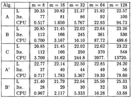
Mizuno, A. Yoshise & T. Kikuchi

Table 1. Computational results for Problem 1

Alg. m

=

8 m

=

16 m

=

32 m

=

64 m

=

128 L 20.33 20.82 21.37 21.92 22.57 A Ite. 77 81 86 92 100 CPU 0.517 1.650 5.767 22.93 94.73 L 20.85 21.45 22.02 22.64 23.26

B

Ite. 112 166 245 361 530 CPU 0.700 3.167 16.10 87.72 499.6 L 20.85 21.45 22.02 22.62 23.22 C Ite. 112 166 250 370 548 CPU 3.700 31.62 244.8 2077. 13720. L 22.77 22.14 22.50 22.85 24.20 A' Ite. 37 40 44 49 56 CPU 0.717 1.783 5.367 19.30 78.60 L 21.40 21.79 22.04 25.50 25.33

B'

Ite. 28 29 30 32 33 CPU 0.967 2.117 5.333 16.28 53.88

Table 2. Computational results for Problem 2

Alg. m

=

8 m

=

16 m

=

32 m

=

64 m

=

128 L 21.43 22.16 22.98 24.01 24.87 A Ite. 81 85 90 96 102 CPU 1.033 5.017 31.33 222.8 1746. L 21.89 22.78 23.64 24.57 25.48

B

Ite. 118 177 264 393 582 CPU 1.400 10.22 89.57 914.7 10110. L 21.89 22.78 25.70 24.56 25.47 C Ite. 118 177 270 404 605 CPU 3.983 34.15 259.3 2135. 14990. L 24.29 22.70 25.87 24.69 25.72 A' Ite. 41 44 49 53 58 CPU 1.100 3.883 20.62 136.4 1064. L 24.67 25.43 26.54 27.35 25.58

B'

Ite. 32 34 36 38 39 CPU 1.317 3.917 17.13 101.6 713.1

Table 3. Computational results for Problem 3 Alg. m

=

8 m

=

16 m

=

32 m

=

64 m

=

128 min. 19.55 20.00 21.25 22.02 L aye. 19.90 20.69 21.54 22.23 23.16 max. 20.08 20.99 21.72 22.38 min. 74 79 84 90 A Ite. aye. 74.9 7!l.5 84.7 90.5 99 max. 76 80 85 91 min. 0.917 4.683 29.30 208.9 CPU aye. 0.977 4.800 29.79 212.9 1739. max. 1.050 5.050 30.18 217.6 min. 20.27 20.98 21.76 22.51 L aye. 20.51 21.18 21.89 22.62 23.47 max. 20.71 21.41 22.03 22.70 min. 109 162 242 359 B Ite. aye. 110.1 164.1 243.4 360.7 535 max. 112 166 245 362 min. 1.283 9.400 82.93 836.8 CPU aye. 1.362 9.465 83.59 864.1 9712. max. 1.400 9.567 84.43 980.8 min. 20.27 20.98 21.71 22.49 L aye. 20.51 21.21 21.87 22.66 23.47 max. 20.71 21.41 21.97 22.69 min. 109 162 246 368 C Ite. aye. 110.1 164.1 247.8 370.1 554 max. 112 166 249 371 min. 3.633 30.77 245.7 2084. CPU aye. 3.885 31.17 248.8 2110. 13780. max. 4.430 3153 250.8 2124. min. 20.46 20.56 21.31 22.30 L aye. 21. 72 22.03 22.22 22.74 23.97 max. 22.66 2377 23.75 23.81 min. 36 40 44 50 A' Ite. aye. 37.4 42.2 45.9 51.4 58 max. 40 43 48 52 min. 0.950 3.600 18.63 127.2 CPU aye. 1.010 3.818 19.66 132.8 1053. max. 1.133 3.983 20.53 136.1 min. 20.49 22.02 21.83 22.54 L aye. 21.76 22.53 22.92 23.08 24.42 max. 22.95 24.39 24.17 23.77 min. 27 31 32 35 B' Ite. aye. 29.3 32.1 33.5 35.5 37 max. 30 33 35 36 min. 1.117 3.483 15.15 93.33 CPU aye. 1.202 3.688 16.00 94.91 678.9 max. 1.267 3.810 16.58 96.33

88 logz I 5 4 3 2 1

s.

Mizuno. A. Yoshise & T. Kikuchi

k

100 200

Fig.1 Graph of (k, IOglO

<

Xk, yk

»

for Problem 1

2

o

-1 -2 -3 -4 -5 -6 -7 A' _ _ _ _ _ _ _ _ B' 3 4 5 6 7 logzm 3 4 5 6 _{7logz m}

Fig.2 Graph of (log2 m, log2 1) Fig.3 Graph of (lOg2 m, log2 J)

(b) the row lte. shows the iteration number k of the terminated point (Xk, yk),

(c) the row CPU shows the CPU time by second from when we get the initial point until when we get the terminated point,

(d) the row min., ave. and max. in Table 3 show the minimum, average and maximum

values of each data item for 10 examples, respectively.

In each case, an approximate solution is obtained. From Table 1, Table 2 and Table 3, we can see that

(1) Algorithm A is faster than Algorithm B and Algorithm B is faster than Algorithm C,

(2) Algorithm A' accelerates Algorithm A and Algorithm B' accelerates Algorithm B except for small problems.

(3) In Table 3, the difference between minimum and maximum values for each case is very small. So each algorithm is stable with respect to computation time and the number of iterations.

In order to see the way of convergence, we get the data of the values of all < Xk, yk

>

for Problem 1 of m = 32 and illustrate the ,graph of (k, IOg10

<

Xk, yk

»

in Fig.I. We can observe from Fig.1 that

(4) the convergence of each of Algorithms A, Band C is linear,

(5) the convergence of each of Algorithms A' and B' is at least linear and is superlinear when the values

<

Xk, yk

> become sufficiently small.

Though we here omit the figures for Problem 2 and Problem 3, we get the same obser-vations as (4) and (5).

We see in section 3.4 that the iteration number is at most O( ne L1 ) for c = 1

(Algorithm A) or c = 0.5 (Algorithm B and Algorithm C), and the number of arithmetic operations per iteration is at most O(nd_{) for d = 3 (Algorithm A and Algorithm B) or}

d

=

2.5 (Algorithm C). So we consider that the following values

I

=

(data in lte.)/(data in L)

and

J = (data in CPU)/(data in lte.)

will be in proportional to some exponential of the problem size m for each problem and each algorithm, i.e., there are c and d such that

90 S. Mizuno, A. Yoshise & T. Kikuchi

J is proportional to mC

and

J is proportional to md•

Then we say that the practical computational complexity of iteration numbers is O( mC _L

1 ), the practical computational complexity per iterations is O( md) and the

practical computational complexity is O(mc₊d

_Ld.

In order to guess the values of c and d for Problem 1, we draw the graph of (IOg2 m, log2 J) in Fig.2 and the graph of (IOg2 m, log2 J) in Fig.3. It will be found that the data for each algorithm almost lay on a straight line in each of Fig.2 and Fig.3. So we estimate the values of c and d as the gradients of regression lines of the data. In the same way, we get the estimate values of c and d for Problem 2 and Problem 3. We show the obtained estimate values in Table 4, where we also put the theoretical upper bounds which are given in Section 3.4.

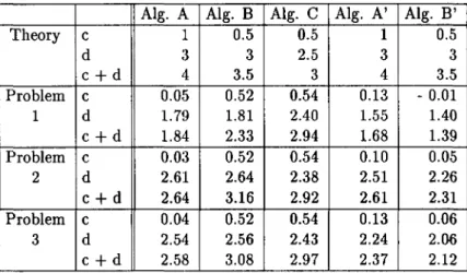
Table 4. The estimation of c and d

Alg. A Alg. B Alg. C Alg. A' Alg. B'

Theory c 1 0.5 0.5 1 0.5 d 3 3 2.5 3 3 c+d 4 3.5 3 4 3.5 Problem c 0.05 0.52 0.54 0.13 - 0.01 1 d 1.79 1.81 2.40 1.55 1.40 c+d 1.84 2.33 2.94 1.68 1.39 Problem c 0.03 0.52 0.54 0.10 0.05 2 d 2.61 2.64 2.38 2.51 2.26 c+d 2.64 3.16 2.92 2.61 2.31 Problem c 0.04 0.52 0.54 0.13 0.06 3 d 2.54 2.56 2.43 2.24 2.00 c+d 2.58 3.08 2.97 2.37 2.12

From Table 4, we can see that

(6) The values of c for each algorithm are almost the same in Problem 1, Problem 2 and Problem 3. However the values of d for each algorithm except for Algorithm

C are less in Problem 1 than in Problem 2 and Problem 3 (probably because the matrix M of Problem 1 is upper triangular).

(7) The practical computational complexities of Algorithm C are almost the same as the theoretical upper bounds, but those of the other algorithms are less than the theoretical upper bounds.

(8) The values of c in Algorithms A, A' and B' are almost zero. This fact implies that the iteration number is proportional only to L1 but not to m.

(9) The practical computational complexity of Algorithm A is less than those of Al-gorithm B and AlAl-gorithm C for each problem.

(10) The practical computational complexity of Algorithm B' is less than that of Algorithm B for each problem.

6. Conclusions

This paper describes three prototype algorithms (Algorithm A, Algorithm B and Al-gorithm C) and two modified alAl-gorithms (AlAl-gorithm A' and AlAl-gorithm B') for linear complementarity problems. Then we compare the algorithms in theory (Section 3.4) and in practice (Chapter 5). We can conclude that all proposed algorithms are poly-nomial time in theory and in practice, and

Algorithm C

>

Algorithm B Algorithm A

>

Algorithm B Algorithm A'

>

Algorithm A Algorithm B'

>

Algorithm B

>

Algorithm A in theory,

>

Algorithm C in practice, in practice, in practice, where"

>"

means "better than" or "faster than".

Acknowledgment

The authors wish to thank Professor Masakazu Kojima for his useful suggestions, Professor Masao Mori for his warm encouragement to their study and Mr. Isao Ko-hiyama for his help in our computational experiments. They are also grateful to Profes-sor Yoshitsugu Yamamoto for his comment on Theorem 2 and referees for their helpful comments. Part of the research of the first author was supported by Grant-in-Aid for Encouragement of Young Scientists 63731004 of the Ministry of Education, Science and Culture.

92 s. Mizuno, A. Yoshise & T. Kikuchi

References

[1] J. R. Birge and A. Gana. Computational complexity of Vander Heyden's variable dimensional algorithm and Dantzig-Cottle's principal pivoting method for solving LCP's. Mathematical Programming, 26:316-325, 1983.

[2] R. W. Cottle and G. B. Dantzig. Complementary pivot theory of mathematical programming. Linear Algebra and Its Applications, 1:103-125, 1968.

[3] Y. Fathi. Computational complexity of LCP's associated with positive definite symmetric matrices. Mathematical Programming, 17:335-344, 1979.

[4]

N. Karmarkar. A new polynomial-time algorithm for linear programming.

Com-binatorica, 4:373-395, 1984.

[5] M. Kojima, S. Mizuno, and A. Yoshise. A polynomial-time algorithm for a class

of linear complementarity problems. Research Reports on Information Sciences B-193, Dept. of Information Sciences, Tokyo Institute of Technology, Oh-Okayama, Meguro-ku, Tokyo 152, Japan, 1987.

[6]

M. Kojima, S. Mizuno, and A. Yoshise. A primal-dual interior point algorithm for linear programming. In N. Megiddo, editor, Progress in Mathematical

Pro-gramming, Interior-Point and Related Methods, pages 29-47, Springer-Verlag, New York, 1988.

[7] C. E. Lemke. Bimatrix equilibrium points and mathematical programming.

Man-agement Science, 11:681-689, 1965.

[8] K. G. Murty. Computational complexity of complementarity pivot methods.

Mathematical Programming Study, 7:61-73, 1978.

[9] J. S. Pang, I. Kaneko, and W. P. Hallman. On the solution of some (parametric) linear complementarity problems with application to portfolio selection, structural engineering and actuarial graduation. Mathematical Programming, 16:325-347, 1978.

[10] 1. Van der Hyden. A variable dimension algorithm for the linear complementarity problem. Mathematical Programming, 19:328-346, 1980.

[11] Y. Ye. Further development on the interior algorithm for convex quadratic

pro-gramming. Integrated Systems Inc. and Department of Engineering-Economic Systems, Stanford University, Santa Clara, CA 95054 and Stanford, CA 94305, 1987.

Shinji MIZUNO: Department of In-dustrial Engineering and Manegement, Tokyo Institute of Technology