ECCを用いた耐マルチビットソフトエラー高位合成について

全文

(1)DAシンポジウム Design Automation Symposium. DAS2018 2018/8/30. ECC を用いた耐マルチビットソフトエラー高位合成について Inoue Keisuke1,a). Abstract: This paper discusses the Multiple Bit Upset (MBU) problem on Application Specific Integrated Circuit. (ASIC). It focuses especially on the storage part (register) of ASIC since the transient error on registers can be quickly propagated to the other part of the system. It proposes a novel high-level synthesis where a set of registers and error correcting code modules against MBU are grouped to maximize the reliability of ASIC with low cost. It also proposes a heuristic-based algorithm to find optimal data covering, and experimental results to show the effectiveness of the proposed method.. 1. Introduction With the scaling of silicon process technologies into the nanometer regime, the reliability of Application Specific Integrated Circuits (ASICs) becomes a significantly important concern for designers [1]. Nanoscale components such as functional units, multiplexers, and registers themselves are likely to fail often. As ASIC designers integrate more of components onto the processing die, the number and size of registers will increase. Unfortunately, a direct drawback is the increase in the device vulnerability to radiation, as charge particles which were once negligible, become more likely to produce upsets. When charged particles strike the silicon die, they lose their energy, resulting in a dense ionized region. The ionization generates a charge deposition, i.e., a transient current pulse. This effect is called Single Event Upset (SEU). With the downscaling of devices, the physically neighboring bits can sometimes be upset by one particle known as Multiple Bit Upset (MBU). Although SEU is the major concern in ASICs, MBU starts to be also a matter of serious concern to be addressed nowadays with the nanometric technologies [2]. Under the influence of MBU, conventional single-errorcorrecting codes (ECCs) are not sufficient to cope with the expected soft errors. This deficiency motivates to use more stronger ECC schemes, such as Bose-Chaudhuri-Hocquenghem (BCH) code [3], Reed-Solomon code, and Punctured Difference Set. With the advantages of simplifying the programming circuits and maintaining the programming throughput, the use of strong ECC is subject to two main drawbacks[5]: (i) strong ECC induces higher coding redundancy (i.e., larger number of parity bits) that will degrade the storage capacity of registers, and (ii) the ECC decoder will induce area and power overhead. For example, TABLE I shows the specification list of BCH code, where m is a positive integer, n is the code length (n = 2m − 1), k is the number of information bits (n − k is the number of parity bits), and t is the 1 a). International College of Technology, Kanazawa [email protected]. ⓒ 2018 Information Processing Society of Japan. Table 1. BCH code parameters. m. n. k. t. m. n. k. t. 3 4. 7 15. 4 11 7 5 26 21 16 11 6. 1 1 2 3 1 2 3 5 7. 6. 63. 57 51 45 39 36 30 24 18 16. 1 2 3 4 5 6 7 10 11. 5. 31. m. 7. n. 127. k. t. 10 7 120 113 106 99 92 85 78. 13 15 1 2 3 4 5 6 7. error correcting capability (i.e., at most t errors can be fixed). We can see that the higher the error-correcting capability becomes, the larger the number of parity bits becomes. In conventional soft error-aware ASIC design, error-correcting has been considered for each register independently [4]. For example, let us assume that 2-bit errors occur on a silicon die. If using BCH code, a 32-bit register (#information bits is 31) requires 10 parity bits against 2-bit errors. Therefore, two registers require 20 parity bits. Our main idea is to view a group of registers as one register when considering error-correcting. If we can treat two 32-bit registers as one 64-bit register, only 12 parity bits are required against 2-bit errors (8 parity bits can be saved) without loss of the error-correcting capability. We can expect the power reduction because an ECC decoder executes for several registers at a time. In this paper, we propose a novel ECC-based high-level synthesis (HLS) that can be continue to operate in the presence of multi-bit transient errors. This paper makes the following contributions: • It proposes a new register system with an ECC module against MBU, where some registers are grouped, and ECC computing/error-checking/error-correcting are performed for these registers. • It introduces a new concept of cover that consists of (a set of data, time-interval). The set of data in a cover are errorchecked and corrected together during the time-interval. A 75.

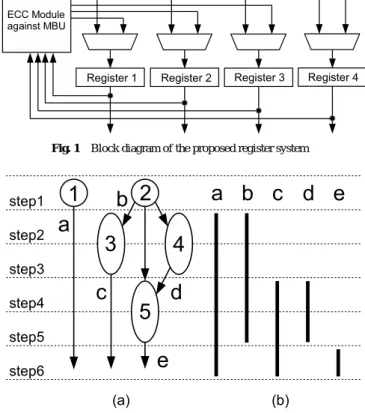
(2) DAシンポジウム Design Automation Symposium. DAS2018 2018/8/30. cover is an intersection of data-lifetimes. • In general, more than one covers would be required. Different covers produce different reliability capabilities. Therefore, this paper introduces a new HLS task, namely cover assignment which chooses a cover pattern, and formulates a problem to find an optimal cover assignment. • It proposes a heuristic-based cover assignment algorithm to maximize the coverage ratio, and shows experimental results. This paper is organized as follows: The next section presents the discussion of prior works. Section III presents our design framework, a motivational example of our optimization problem, and a heuristic-based algorithm to solve it. Experimental results are shown in Section IV. Finally, Section V concludes the paper.. Fig. 1. Block diagram of the proposed register system. 2. Related Works Various techniques have been developed over the past few years to make the ASIC reliable [6], [9]. In physical level, standard CMOS technology typically fails due to radiation-induced leakage currents in the field oxide region. Recent work suggests that spatial multi-bit errors are increasingly likely at future technology nodes. As other techniques for memory, bit interleaving is the promising approach used to protect memory arrays from spatial multi-bit errors [7]. Modern microprocessors and ASICs already use various protection techniques such as ECC, and hardware redundancy to safeguard their register system. A common technique to protect memory arrays against errors is to use error detecting codes and ECC. ECC is typically applied to the data on a per-word basis and allows error detection/correction at the cost of extra bits of code storage per word and shared calculation/checking/correction logic. The extra area and energy overhead to implement multi-bit error detection and correction codes grows quickly as the code strength is increased [8]. Furthermore, scaling up conventional techniques to cover multi-bit errors will incur large performance, area, and power overheads in part due to the tight coupling between the error detection and correction mechanisms.. 3. MBU Hardening Design High-level synthesis (HLS) is the process of translating a behavioral description into a register-transfer-level structure description. In this paper, we focus on HLS, and discuss MBUaware register system to avoid transient error-induced malfunction. 3.1 ECC-Based Register System against MBU Figure 1 shows the block diagram of our register system with an ECC module and four registers (The proposed architecture allows any ECC system). In this system, the output terminals of the registers are connected to the input of ECC module. Normally, a register operates in the same manner as an ordinal register. When computing parity bits, ECC module collects all the outputs, and distributes the resultant parity values to the registers. Error checking and correcting are performed periodically (e.g., once every 2steps). Note that register grouping can be changed using multiplexers and wires during ASIC operation. ⓒ 2018 Information Processing Society of Japan. Fig. 2. (a) An example scheduled DFG, and (b) a set of data-lifetimes.. 3.2 Mathematical Model Basis of HLS: A data flow graph (DFG), behavioral description of HLS, is given as a directed graph G(O, A), where the vertex set O = {i | i = 1, 2, . . . , } represents the operations in the DFG and the arc set A represents the data dependencies between operations. The time axis is divided by the rising-edge of the clock signal, and each divided timing is referred to as step. Operation scheduling is an HLS task to assign each operation to a step. Figure 2(a) shows an example DFG and a scheduling result where, for example, operation 1 is scheduled at step 1. The datalifetime of data a is defined as the open interval on the time axis from the step at which a is generated, and to the last step where a is consumed by other operations. Figure 2(b) shows a set of data-lifetimes represented as bold vertical lines. For example, the data-lifetime of data b is the open interval from step 2 to step 5 since b is generated at step 2, and lastly referred by operation 5 at step 5. Two data with no data-lifetime overlapping can share the same register. Cover: Given a set of data, we introduce a new concept of cover which is an intersection of the data-lifetimes of the data. The meaning of cover is that the data in a cover are protected by one ECC code (ECC code must be re-computed if the stored data are changed). For example, a shaded region with respect to data a and b in Fig. 3(a) is a cover. At the beginning of step 2, two registers storing a and b are grouped and connected to ECC module in a same way with Fig. 1, and ECC is computed. By the end of step 5, error checking and correcting are periodically performed for a and b. Cover assignment: The register system is constructed for each cover. The relevant registers are grouped at the beginning of a cover, and released after the end of the cover. We can realize 76.

(3) DAシンポジウム Design Automation Symposium. DAS2018 2018/8/30. tionate to the number of required registers. Therefore, it is better to reduce the maximum number of temporal cover overlaps. (3) The coverage ratio: To protect data against MBU, every data should be included in a cover. However, as shown in the next section, it could be not always achieved in general. Therefore, we define a design measure the coverage ratio which is the total number of covered data-lifetime length, divided by the total number of data-lifetime length. It is better to maximize the coverage ratio to enhance the MBU tolerance. Fig. 3. Two different cover results. (a) is obtained by a greedy method, and the coverage ratio is 0.86. (b) is the optimal result with the coverage ratio 1.00. Note that data e is ignored due to the minimum interval constraint.. such a variable system using multiplexers, wires, and control signals. Since a cover is an intersection of data-lifetimes, all the data cannot be included to one cover in general. As shown later, different covers produce different results due to the various design constraints (described in the next section). We introduce a new HLS task namely the cover assignment that decides the covers on data. 3.3 Design Constraints The following basic constraints can be considered in the proposed design. The minimum interval constraint: We assume that the errorchecking interval is given as a design input. We can exclude the data whose data-lifetime lengths are smaller than the errorchecking interval since they are never checked. For example in Fig. 2(b), if the error-checking interval is 2, data e can be ignored when considering cover assignment because the datalifetime length of e is smaller than 2. The maximum cover width constraint: We call the number of data in a cover as cover width. The maximum cover width is limited by a hardware constraint which is given as a design input. Note that each cover width can take any value no larger than the maximum cover width α. If the cover width is less than α, dummy data are padded so as to make the cover width equal to α. The minimum cover length constraint: The time length of a cover must be larger than or equal to the error-checking interval due to the same reason with the minimum interval constraint. 3.4 Design Objectives The following basic objectives can be considered in the proposed design: (1) The number of covers: It is known that computing ECC code for MBU induces large power cost [5]. For each cover, ECC is computed at the beginning of the cover. Therefore, the number of covers is the same with the number of computing ECC codes. To reduce power overhead, it is better to reduce the number of covers. (2) The maximum number of temporal cover overlaps: The maximum number of temporal cover overlaps is proporⓒ 2018 Information Processing Society of Japan. 3.5 Motivational Example As the first objective targeted in the proposed design, we choose objective (3), the coverage ratio, because the most important aim of the design is to protect data against soft-errors. We treat the other objectives (1) and (2) as design constraints in the paper. Let us take Fig. 2(b) as an example. We assume the following design constraints: the minimum interval is 2, the maximum cover width is 2, the minimum cover length is 2, the maximum number of covers is 3, and the maximum number of temporal cover overlaps is 2. Data e is ignored due to the minimum interval constraint. First, let us consider a simple greedy algorithm such that a set of data are greedily covered in order of the start time of data-lifetimes. As a first step, we choose data a and b, and cover them as long as possible. So the first cover is a set of a and b with the time interval from step 2 to step 5. Note that step 6 is not included in the cover since a cover is an intersection of data, and the data-lifetime of b ends at step 5. Next, we choose data c and d, and cover them as long as possible. So the second cover is a set of c and d with the time interval from step 4 to step 5. The resultant cover solution is shown in Fig. 3(a) (Note that data a and c in step 6 cannot be covered due to the minimum cover length constraint). The coverage ratio is computed as 0.86 (=12/14) since the total number of covered data-lifetime length is 12, and the total number of data-lifetime length is 14. However it is not optimal. The optimal solution is shown in Fig. 3(b). In this solution, all the data are covered, and then the coverage ratio is 1.00. This observation motivates us to develop a covering algorithm to maximize the coverage ratio. We explain hardware operations based on the cover result in Fig. 3(b). At the beginning of step 2, a register system with two registers storing a and b, and an ECC module, is constructed. ECC is computed (the resultant parity bit values are distributed to the registers), error checking and correcting are periodically performed in the register system. This register system is released at the end of step 3. At the beginning of step 4, register systems for two registers storing c and a (b and d) are constructed in a same way. ECC is computed, error checking and correcting are periodically performed in the register systems by the end of step 6. Note that these hardware operations do not depend on register assignment (an HLS task assigning data to registers). So we focus on the cover assignment in the paper. 3.6 Problem Formulation The objective of our design is to find a set of covers that maximizes the coverage ratio under the design constraints described 77.

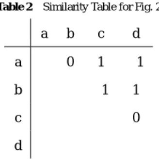
(4) DAシンポジウム Design Automation Symposium. in Sects. 2-C and D. The constrained HLS problem we want to solve in the paper can be formulated as: Problem: Under a given resource set and an operation scheduling result, find a set of covers such that (i) the minimum interval constraint, the maximum cover width constraint, and the minimum cover length constraint are satisfied, (ii) the number of covers, and the maximum number of temporal cover overlaps is no larger than the designated values, and (iii) the coverage ratio is maximum. The computational complexity of our problem is unknown at this point. However we expect that it is a difficult problem because a similar problem, the graph vertex cover problem is NPhard. In this paper, we propose a heuristic algorithm to efficiently find sub-optimal solutions in the next section. 3.7 A Heuristic-based Covering Algorithm The objective of our cover assignment is to find a set of covers that maximizes the coverage ratio under design constraints. First, we show a cover assignment algorithm in case that the maximum cover width is 2 which will be extended for general cases later. To choose a pair of data that will be assigned to a cover, we focus on a similarity of data. One possible reason to result in uncovered parts of datalifeitmes is the temporal difference of paired data. For example in Fig. 3(a), the temporal difference between data a and b is 1 which is less than the minimum cover length 2. After making a cover for these data, a small part of data-lifetime (the data-lifetime of a in step 6) remains not to be covered. Therefore, it is unpreferable to choose such a data pair. To all the pair of data, we add −∞ point if they have no lifetime overlapping. We add −1 point if they satisfy the following conditions (We add −2 points if they satisfy both of the constraints): • The difference of the start time of the data-lifetime is less than the error-checking interval. • The difference of the end time of the data-lifetime is less than the error-checking interval. If the start and/or end time of data-lifetimes are same, it is preferable to make them a pair. To all the pair of data, we add 1 point if they satisfy the following conditions (We add 2 points if they satisfy both of the constraints): • The start time of the data-lifetime is the same. • The end time of the data-lifetime is the same. TABLE 2 shows similarity values for the data in Fig. 2(b) under the condition that the minimum cover length is 2. For example, a and b have the same start time, so this pair takes 1 point. However, the difference of their end times is less than the minimum cover length. So this pair takes −1 point, and the total point is 0. a and c have the same end time, so this pair takes 1 point. The difference of their end times is no less than the minimum cover length (no point down). So the total point is 1. For a and d, the difference of their end times is less than the minimum cover length. So this pair takes −1 point. The difference of their start times is no less than the minimum cover length (no point down). So the total point is −1. The following summarizes our algorithm. Step 1 Compute the similarity table like TABLE 2 ⓒ 2018 Information Processing Society of Japan. DAS2018 2018/8/30. Table 2 Similarity Table for Fig. 2. a a. b. c. d. 0. 1. −1. −1. 1. b c. 0. d. Step 2 Choose a pair with the highest similarity value. If two pairs have the highest value, choose one pair arbitrarily. Step 3 Assign them to a cover as long as possible unless violating the maximum cover width constraint and the minimum cover length constraint. Step 4 Remove the covered parts of data-lifetimes when computing similarity. Step 5 If there is no possible pair to be covered, output all the covers, and finish algorithm. Otherwise, return back to Step 1. We illustrate the algorithm by applying it to Fig. 2(b). In TABLE 2, there are two pairs that have the highest similarity value ({a, c}, {b, d}). We choose {a, c}, and assign a cover to them as long as possible. Figure 4-left shows this cover, and Fig. 4-right shows the updated similarity value table after the covered parts are removed. Since whole data-lifetime of c is covered, c is removed from the table. The uncovered part of a and b have the same start time, so this pair takes 1 point. The difference of their end times is no less than the minimum cover length (no point down). So the total point is 1. The uncovered part of a and d have no data-lifetime overlap. So the similarity value of them is −∞. The similarity value of b and d is the same with TABLE 2. We choose {a, b}, and assign a cover to them as long as possible. Figure 5-left shows this cover, and Fig. 5-right shows the updated similarity value table after the covered parts are removed. Since whole data-lifetime of a is covered, a is removed from the table. The uncovered part of b and b have the same start time and end time, so the total point of this pair is 2 points. We choose {b, d}, and assign a cover to them as long as possible. After that, since there is no possible candidate data, the algorithm is finished. The final covering result is the same with Fig. 3(b). In this case, the proposed algorithm achieves the optimal result with the coverage ratio 1.00. It is clear that our algorithm works in a polynomial time. 3.8 Extending the Proposed Algorithm to General Cases We can easily extend this algorithm to treat the case that the maximum cover width is larger than 2. For example, the maximum cover width is 3, the similarity of three data is computed by the average of the similarity of every pair chosen from them. The algorithm computes the similarity to every combination of three data in Step 1.. 4. Experimental Results 4.1 Setting We applied the proposed algorithm to an HLS benchmark circuit. Only two types of operations, addition and multiplication 78.

(5) DAシンポジウム Design Automation Symposium. DAS2018 2018/8/30. Table 3. a a. b. d. 1. −∞. Design. LEN.. WIDTH=2 (#cover). WIDTH=3 (#cover). Greedy. 2. 109/119=0.92 (15). 108/119=0.91 (13). 3. 97/111=0.87 (8). 94/111=0.85 (9). 4. 88/99=0.89 (8). 79/99=0.80 (7). 5. 82/91=0.90 (6). 73/91=0.80 (4). 1. b d. Ave. Prop.. Fig. 4. After the first iteration of the algorithm, a and c are covered during the time between step 4 and step 6.. b. d 2. d. Fig. 5. After the second iteration of the algorithm, a and b are covered during the time between step 2 and step 3.. (ADD and MUL, for short), are considered in this experiment. We assume that every operation has one step delay. We used a benchmark the fifth-order elliptic wave digital filter (EWF) with 34 operations to evaluate the proposed algorithm (it is a middlesize benchmark circuit). We used list-scheduling to compute the operation scheduling result. We evaluated the following two designs for comparison: • Greedy: Greedy algorithm-based design, where cover assignment is performed such that a pair of data is greedily chosen in order of the start time of the data-lifetime (Sect. III-E). • Prop.: The proposed design where the cover assignment result computed by the proposed algorithm (Sect. III-G). 4.2 Results TABLE III shows the experimental results, where LEN. is the minimum cover length, WIDTH is the maximum cover width, #cover is the number of covers, and Ave. is the average of the coverage ratio. For example, for the proposed design with LEN.=2, the total number of data-lifetime length is 119, and the total number of covered data-lifetime length is 118. Therefore, the coverage ratio is computed as 118/119=0.99. We performed experiments if WIDTH=2 and =3. Note that although the maximum cover width is 2 x if using BCH, the proposed design accepts any ECC system. For all the cases, the proposed design achieved better solutions compared with the greedy-based design (6% on average). The computational time is almost zero for all the instances. ⓒ 2018 Information Processing Society of Japan. 0.90. 0.84. 2. 118/119=0.99 (16). 113/119=0.95 (13). 3. 105/111=0.95 (11). 104/111=0.94 (10). 4. 94/99=0.95 (8). 87/99=0.88 (7). 5. 87/91=0.96 (6). 74/91=0.81 (5). 0.96 (+0.06). 0.90 (+0.06). Ave.. b. Coverage Ratio Comparison. 4.3 Discussion For all the cases, the coverage ratio for WIDTH=3 was lower than the case of WIDTH=2. The main reason is that the larger the data group size (cover width) becomes, the smaller the number of similar data becomes. In this experiments, we do not constrain the number of covers. For all the cases, the number of covers used in the proposed design is slightly greater than or equal to greedy-based design. It might be reasonable power penalty to achieve the better coverage ratio. Further investigation is left as an future work. 4.4 Power Overhead Comparison with Conventional Design Using the proposed design, power overhead with respect to ECC computing is expected to be reduced. In conventional design, the number of ECC computing equals to the number of data. TABLE IV shows the number of data in the conventional design (denoted by Conv.). Note that the larger LEN becomes, the smaller the number of data due to the minimum interval constraint. In the proposed design, the number of ECC computing equals to the number of covers. In TABLE IV, x(y, z, w) represents the power overhead of the proposed design where x is the number of covers, y = 1.3 ∗ x, z = 1.4 ∗ x, and w = 1.5 ∗ x (x, y, z, w represents the power overhead normalized by the conventional design). We can see that if the required power of ECC computing for WIDTH=3 is less than 1.5 times of ECC computing for WIDTH=2, the proposed design can reduce the power overhead for most of the cases. Further investigation is also left as a future work.. 5. Conclusion This paper presented a high-level design to protect registers against MBU based on a new concept of cover. The main idea is to view a group of registers as one register when considering error-correcting. As a result, the parity bits for ECC can be reduced with out loss of error correcting capability. We formulated a novel cover assignment problem of optimizing the coverage ratio. We proposed a heuristic-based cover assignment algorithm which was evaluated by experiment supporting the effectiveness of our approach. Experiments compared the proposed design with the greedy-based design. It is important to apply the pro79.

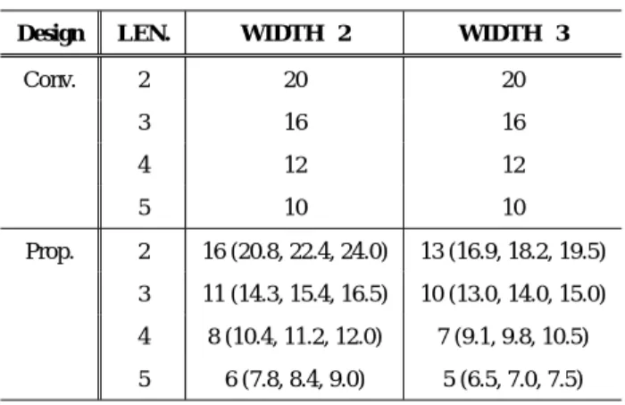
(6) DAシンポジウム Design Automation Symposium. Table 4. DAS2018 2018/8/30. Power Overhead Comparison. Design. LEN.. WIDTH=2. WIDTH=3. Conv.. 2. 20. 20. 3. 16. 16. 4. 12. 12. 5. 10. 10. 2. 16 (20.8, 22.4, 24.0). 13 (16.9, 18.2, 19.5). 3. 11 (14.3, 15.4, 16.5). 10 (13.0, 14.0, 15.0). 4. 8 (10.4, 11.2, 12.0). 7 (9.1, 9.8, 10.5). 5. 6 (7.8, 8.4, 9.0). 5 (6.5, 7.0, 7.5). Prop.. posed design to various types of benchmark circuits. References [1] [2] [3] [4] [5] [6] [7] [8] [9] [10]. K. Agarwal, ”Characterizing process variation in nanometer CMOS,” Proc. ACM/IEEE DAC, pp. 396–399, Jun. 2007. M.Maniatakos, M.K.Michael, and Y.Makris, ”Vulnerability-Based Interleaving for Multi-Bit Upset (MBU) Protection in Modern Microprocessors,” Proc. ITC, paper. 19.2, May 2012. S. Lin and D. Costello, Error Control Coding: Fundamentals and Applications, Prentice-Hall, Englewood Cliffs, NJ, 2004. A. Hossein and M.B. Tahoori, ”Soft error modeling and remediation techniques in ASIC designs,” Volume 41, Issue 8, pp. 506–522, August 2010. W.Wu, ”MBU-Calc: A compact model for Multi-Bit Upset (MBU) SER estimation,” Proc. IRPS, 2015. J. Maiz, S. Hareland,K.Zhang, and P.Armstrong, ”Characterization of multi-bit soft error events in advanced SRAMs,” Proc. EDM, 2004. S. Baeg, S. Wen, and R. Wong, ”SRAM Interleaving Distance Selection With a Soft Error Failure Model,” IEEE Transactions on Nuclear Science, Volume: 56, Issue: 4, Aug. 2009. R. Naseer and J. Draper, ”DEC ECC design to improve memory reliability in Sub-100nm technologies,” Inter national Conference on Electronics, Circuits and Systems, 2008. R.C. Baumann, ”Radiation-induced soft errors in advanced semiconductor technologies”, IEEE Transactions on Device and Materials Reliability, vol. 5, no. 3, pp. 305-316, 2005. G.Neuberger, ”A Multiple Bit Upset Tolerant SRAM Memory,” ACM TODAES, pp. 577–590, 2003.. ⓒ 2018 Information Processing Society of Japan. 80.

(7)