The Lexico-Bounded Flow Algorithm for Solving the Minimum Cost Project Scheduling Problem with an Additional Linear Constraint

Society of Japan

Vo!. 27, No. 3, September 1984

THE LEXICO- BOUNDED FLOW ALGORITHM FOR SOLVING

THE MINIMUM COST PROJECT SCHEDULING PROBLEM

WITH AN ADDITIONAL LINEAR CONSTRAINT

Takashi Kobayashi

Saitama University

(Received November 4,1983: Revised March 21,1984)

Abstract This paper proposes an algorithm for solving the minimum cost project scheduling problem with an additional linear constraint whose right hand side is a parameter. Instead of putting the additional constraint, we add it to the objective function, where it is multiplied by a parameter. First, we get an optimal solution when a parameter is zero, and next, increase it to infinity. To do so, we iterate to fmd two dimensional flow on the given arrow diagram. The bounds for each arrow flow are determined by the current solution. The first elements are related to the costs, and the second to the coefficients in the additional constraint. A lexico-bounded flow is defmed as the flow such that each arrow flow is within the bounds in the lexicographical ordering. When a lexico-bounded flow exists, the parameter is increased. Otherwise, the function of the additional constraint is increased. Our algorithm is almost dual to the lexico-shortest route algorithm for the minimum cost flow problem with an additional linear constraint. For example, a loop is replaced by a cutset. Our algorithm is also applicable to a pro-ject scheduling problem with two obpro-jectives by combining them with a parameter.

1.

Introduction

The project scheduling problems with additional linear constraints occur when there exist divisible activities or when some activities use a common resource, and some algorithms are presented for getting the length of critical path [6, 8, 9, 11]. This paper presents an algorithm for solving the minimum cost project scheduling problem with an additional linear constraint, whose right hand side is a parameter. The author has presented an algorithm for the minimum cost flow problem with an additional linear constraint, called the lexico-shortest route algorithm [10]. By transforming it in the dual way, like replacing a loop by a cutset, we get our algorithm.

Let

n(t);;;e

be the additional constraint, where

e

is a parameter. Instead of putting it, we add $·n(t) to the objective function, where $ is a parameter. First, we get an optimal solution for $=0, and next, increase $ to infinity. To do so, we iterate to find two dimensional flow on the given arrow diagram. The bounds for each arrow flow are determined by the current solution. The first elements are related to the eosts, and the second to the coefficients in

net).

A lexico-bounded flow is defined as the flow such that each arrow flow is within the bounds in the lexicographical ordering. When a lexico-bounded flow exists, $ is increased. Otherwise,

net)

is increased. We prove the validity of our algorithm by the complementary slackness conditions.

2. Problem Formulation

Let us consider an arrow diagram for a project, with n nodes, numbered 1, 2, ... , n, where node 1 represents the st.art and node n the termination. Let A be the set of jobs (pairs of nodes), and for each job (i,j), the standard time

h . . , and the shortest time g . . are given, where h .. ;;;g... Furthermore, for

~J ~J ~J ~J

(i,j) such that h .. >g . . , the cost for shortening the time

~J ~J by a unit c .. is ~J

given. Conveniently, let c .. =0 for (i, 'i) such that h .. =g . . '

~J - ~J ~J Then, the minimum

cost project scheduling problem with an additional linear constraint is formu-lated as follows:

PO(e):

Minimize zO(t) L c . . (h .. -t .. ) (i,j) ~J ~J ~J subject to (2.1) g .. ~

t ..

~ h .. « i , j)t;A) " ~J ~J ~J (2.2) v. +

t ..

~ v. «i,j)£A)., ~ ~J ] (2.3) v

-

v 1

= PO'

n (2.4) L b ..

t ..

;;;

_e,

(i,j) ~J ~J

where

Po

(total duration) is a given po:>itive number, and

e

is a parameter. We assume that b . . ;;;0 for any (i,j)£A, and that b . . =0 for (i,j) such that h . . =

~J ~J ~J

g . . '

Now, let

n(t)= L b .. t .. , (i,j) ~J ~J

and we shall consider the following parametric programming problem with a para-meter ~ instead of 8. P(~): Minimize z(t,~)

=

zO(t)-~n(t) subject to (2.1), (2.2) and (2.3). Let for (i,j)e;A. Then, where

Co

is a constant.

Hence, p(~) is a normal minimum cost project scheduling problem when ~ is fixed. The relations between the solutions of two problems are stated 'by the following theorems.

Theorem

1. Let (~,t) be an optimal solution of P(O). Then it is also optimal to P

O(8) for any 8 such that 8~n(t).

Theorem

2. Let (~,t) be an optimal solution of P(~) for some positive ~. Then it is also optimal to PO(n), when n=n(t).

It is proved in the same way as theorem 2 of [10J.

3. Dual problem and Complementary Slackness Conditions

We consider the dual problem to P(~).

D(~): Maximize w

=

_{-PO·q-LhijX: j} +

LgijX~j+cO

subject to

0.1)

LX .. -Lx .. j ~J j J~ + x .. +x .. -X . . ~J ~J ~J + x ij ' x ij ' x ij where

Co

is a constant. (i=1), (i=2,3, ... ,n-l), (i=n) , «i,j)r;A) , ;;; 0 «i,j)r;A) ,

Note that q is a variable. Now, we add an arrow (n,l) conveniently, and let

A*=AU{(n,l)}. By replacing q with x

(3.2)

It means

(3.3)

EX .. -Ex .. =O

j ~J j J~ (i=1 ,2, ... .• n).

that (x . . ) is a circulation flO1 •• ~J + = max(c1j(~)-Xij'0), x .. ~J x ..

=

max(x .. -c'!" .(~) ,0), ~J ~J ~J

In any optimal solution,

are satisfied for any (i,j)£A.

The complementary slackness conditions for P(~) and D(~) are as follows: For any (i,j)£A,

(3.4) [ X, .(v .-v .-t . .)=0, ~J J ~ ~J + x .. (t .. -h .. )=0, ~J ~J ~J x -:-.(t .. -g .. )=0. ~J ~J ~J

In any optimal solution, (3.5) t .. = min(v.-v.,h . .)

~J J ~ ~J

is satisfied. Let

Apl {(i,j)

I

(i,j)£A, Ap2 {(i,j)

I

(i,j)£A, (3.6)

Ap3 {(i, j)

I

(i ,j)£A, Ap4 {(i,j)

I

(i,j)£A,

vFvi>h_{i j}} , v .-v .=h . . >g . .},

J ~ ~J ~J

hi/Vj-Vi>gi} , vj-vi=gi} •

Then, (3.4) is replaced by the following

0.7).

(See [5].)

x .. =0 for (i,j)£A_{p1 '} ~J (3.7) O~xiiCij(~) for (i,j)£A_{p2 '} x .. =c . '!"(~) for (i,j)£A_{p3 '} ~J ~J x .. <:c.'!"(~) for (i,j)£A_p4· ~J ~J Next, we let

Adl {(i,j)

I

(i,j)£A, x . . _~J =O),

(3.8) Ad2

{(i,j)

I

(i,j)£A, O<x .. <c.'!"(~)},

~J ~J

Ad3 {(i,j)l(i,j)£A, Xij=cij(~)}, Ad4 {(i,j)

I

(i,j)£A, x .. >c ~J 1.J '!"(~)},

Then, (3.4) can be replaced by the following (3.9) , too.

v .-v.ii;;h .. for (i,j)£A d1, ] 1. 1.]

V .-V .=h .. for (i,j)£A_{d2 '}

(3.9) ] 1. 1.]

hilVj-Vi~gij for (i, j) £A d3,

vj-vi=gij for (i,j)£A_d4·

4. Lexico-bounded Flow

Suppose that we have an optimal solution of P(~),

(v,t).

Let us show that

(v,t)

is optimal to P(~) for some ~>~, or that an optimal solution of P(~) such that

n(t»n(t)

exists.

*

We assign two dimentional real ~ .. for each arrow (i,j)£A. Its upper 1.]

bound CL • • and lower bound i3 .. are determined by Table 1.

1.] 1.J Table 1. (i ,j) CL i j i3i j in Ap1(Vj-vi>hij) (0,0) (0,0)

*

-in A 2 (v .-v .=h . . >g . . ) p J 1. 1.J 1.] (c .. 1.J (~),b 1.J . .) (0,0) in Ap3(hi/Vj-vi>gij) (c ,j(~) ,b .. ) 1. 1.J (cij(~),bij) in A 4

(v

.-v .=g .. ) p ] 1. 1.J (00,00) (c 1.] .,,:(~) ,b.} 1. (n, 1) (00,00) (0,0)

Definition 1.

(~

. .)

is called a lexico-bounded flow (LB flow) i f it 1.J

satisfies the following conditions: (a) L~ . . -L~ .. =0

j 1.J j J1.

(i=1 ,2, ... ,n).

(b) For each (i,j)£A, ~ .. is not greater than CL • • and is not less than i3 .. in

1.] 1.] 1.]

the lexicographical ordering.

Hereafter, we use the lexicographical ordering. and

i3~~)

(k=1,2) represent the k-th elements of

1.]

First, we shall consider the condition for Let

N={l, 2, ... ,

n}.

For any subset of N, say NO' let

(k) (k) Furthermore, let ~.. , CL •• 1.J 1.] ~ •• , CL • • and i3 .. respectively. 1.] 1.J 1.] existence of an LB flow.

and + -C (NO,N O) .-' C-(NO,N O)

*

{U,j)IU,j)EA, iE:N_O' JENO}'

*

{(i,j)

I

(i,j)EA , iE:N

O' JENO}'

C(NO,N

O) = (C+(NO,NO)' C-(NO,NO))' where NO=N-N

O' C(NO,NO)' is called a cutset separating NO and NO (with the direction from NO to NO)'

For a cutset C(NO,N

O)' Y(NO,NO) is defined by Y(NO,N

O) = _(i,j)EC+ L Il, . -_{~J (i,j)cC-}L 13, ., _~J where C+ and C are abbreviations of C+(NO,N

O) and C-(NO,NO) respectively. When a given cutset is obvious, we represent it by y briefly, and let

Theorem 3.

For any cutset C(NO,N

O)" ylf:O.

Proof:

E

+Il~~)

- L

13~~),

(i,j)EC ~J (i,j)EC ~J and there exists (x

ij) that satisfies (3.2) and

1l1~)~Xij~131~)

«i,j)EA),

which is equivalent to (3.7). From the eirculation flow existence theorem [2], Y 1 ~o.

Q.E.D.

Definition 2.

A cutset C(NO,N

O) is called a lexico-negative cutset (LN cutset) if y«O,O).

Theorem

4. An LB flow exist if and only if there exists no LN cutset. Next, we suppose that there exists an LB flow.

Definition

3. The LB flow which maximizes ~nl is called the L-max flow.

Definition

4. The cutset which minimizes

y

among cutsets such that lENO and that nENO is called the L-min cutset"

Theorem

5. ~nl of the L-max flow is equal to

y

of the L-min cutset. This is the max-flow min-cutset theorem Ln the lexicographical ordering.

Let (4.1)

We shall show that we can increase ,p when there exists an LB flow, (~,.),

A2 = {(i,j)I(i,j)£A 2UA 4'

A~l.)·AY.)<O},

p p ~J ~J

and determine ~~1' ~~2' ~~ as follows:

(4.2) min (1) (2) ( ~,J . . ) A £ 1

(-s..

~J IF, .. ), ~J . (1) (2) mm (-A ..

lA . . ),

( . .) A _{~,J £ 2} ~J ~J

If ~(k=l or 2) is empty, let ~~k=oo.

Theorem 6. If there exists an LB flow (F, . . ), for any 0 such that O~O~~~,

~J (;,t) is optimal to P(~+o).

Proof: Let

(4.3) «i,j)£A) •

We shall show that x satisfies (3.7) for ~=~, (v,t)=(;,t).

Every arrow is in one of four subsets A

pk(k=1,2,3,4). Case 1: (i,j)eA p1' As F, . . =(0,0), x .. =0. ~J ~J Case 2: (i,j)£A p2' (0,0) ~ F, . . ~ (c'!". (~), b . .) = (l • . • ~J ~J ~J ~J (2» > (2) (1»

I f F, .. =0, x .. =0 for any

o.

I f

s. .

<0, F,.. 0 and x .. ;;;0 for 0 such that

~J ~J ~J ~J ~J

o~-F, ~

1.) IF,

~~).

Define u .. by

~J ~J ~J (4.4) u .. (c .,,:(~)+ob .. ) _{- x} ij ' ~J ~J ~J Then, u .. A ~ 1.) + CA

~2.)

, ~J ~J ~J and Aij (lij-F,ij;;; (0,0).

I f A

~~\O,

u .. ;;;0 for any C. I f A

~2.\0,

A

~1.»0

and U . . GO for 15 such that

~J ~J ~J ~J ~J

O~-A ~

1.) lA

~2.)

. ~J ~J Case 3: (i,j)£A p3' et .. ~J Hence, x.. c'!" .("$)+cb .. = c'!" .("$+15). ~J ~J ~J ~J Case 4: (i,j)£A p4'

~ .. ;;: (c~J' (~), b . .)

=

S ..•

~J ~ ~J ~J

So, A .. :>(0,0). Define u .. by (4.4).

~J ~J

I f A

~~)~o,

u ..

~o

for any o.

~J ~J I f A ~J

~2.»0,

,\ ~J

~1.)<0,

and u .. ~J

~o

for 0 such that

O:>-A

~

1.)

lA

~~) .

~J ~J

We consider four cases together. TI1en, x defined by (4.3) satisfies (3.7)

for 0 such that o:>o:>~~.

Q.E.D.

Next, assume that there exists an LN cutset, C(NO,N O).

Since a_n1=(oo,oo), 1ENO or nENO. We shall prove that if 1ENO and nEN

O' C(NO,NO)

is also an LN cutset where NO=NO+{n}. Let

and

Then, and

Hence,

Al {(i,n)

I

(i,n)£A, iEN O}

A2

=

{(i,n)1 (i,n)EA, iEN

O}. C+(NO,N O) C+(NO,NO) - Al Y(NO,N_O) = Y(NO,N_O) - La . . - ;~ S .. + Snl < (0,0). A ~J A ~J 1 2

That is, C(NO,N

_O

)

is an LN cutset. From no·w, we do not consider LN cutsets

such that 1ENO and n£N_O.

From theorem 3, y

1=0 and y2<0. Let

Cl {U,j)IU,j)EC+(N

o,No)nAp1}' C

2 {U,j)1 U,j)EC+(NO,NO) n(Ap2UAp3)}' and

C

3 {

U

,j) I

U

,j) EC- (NO,NO) n (Ap3

u

Ap4)}.

Define tw by ~v

(4.5)

min{ min (v.-v.-h . . ), ( . .) C _{~,J E 1} ] ~ ~J min

(v .-v

.-g . . ), ( . .) C ~,J £ 2 ] ~ ~J min (h .. -v .+v.)}. ( . .) C _{~,J E 3} ~J ] ~

Then, we get the following theorem.

Theorem 7. I f there exists an LN cutset C(NO,N

O)' for any E such that

Proof:

Let

x

be an optimal solution of D(~). Then, (v,t)=(v,t) satisfies (3.9) for ~=~, x=x. Let

["

i f _jENO' (4.6) v.

V;-E

] i f je;N

_o'

and ' i j = (

t ..

-E if (i,j)e;C 2, ~J (4.7)

t ..

+t; i f (i,j)e;C 3, ~J

t ..

otherwise. ~J

We show that (v,t) satisfies (3.9) for x=x, too. Since Y1=0,

(1) i f + -x . . =a .. (i,j)e;C (NO,N O) , ~J ~J and (1)

if (i, j) e;C

-

_(NO,NO)' x . . =s ..

~J ~J

+

Therefore, Ad2

n

C and Ad4

n

C are empty. That is, there exists neither (i,j)e;A

d2 with v.-v.<h .. , nor (i,j)e;A] ~ ~J d4 with v.-v.>g ... Hence, (v,t) defined ] ~ ~J

by (4.6) and (4.7) satisfies (3.9) for

x=x,

and it is optimal to P(~). Then,

net)

=

_{net) - E"Y2}

=

net)

+

_Ely2

1.

To hold that v 1=0, let i f je;N

_o'

i f je;N O'

Q.E.D.

5. Lexico-bounded Flow Algorithm

Now, we show our algorithm, called the lexico-bounded flow algorithm (LB flow algorithm). It has two phases. The first phase is for getting what maximizes

n

among optimal solutions of P(O), and the second is for increasing

<I> or n·

LB flow algorithm

Phase 1:

Step 1.

Step 2.

Let t . . =h . . for each (i,j)e;A, and obtain the earliest starting node

~J ~J

time Vj for each*node j. If vn-v1~PO' stop.

For each (i,j)e;A , determine a .. and S .. by table 1, where <1>=0 and

v. is the current value of v .. Find the L-max flow. If it does not

] ]

exist (~n1 is infinite), stop. Step 3. Let C(NO,N

O) be the L-min cutset. Determine ~V by (4.5) and let E=min(~v,vn~O)' and get the new values of (v,t) by (4.6) and (4.7). If Vn=PO(E=Vn-P

O)' go to phase 2. Otherwise, go back to step 2.

Phase 2:

*

Step 1. For each (i,j)EA , determine et

i; and Sij by table. 1. Find an LB flow.

Step 2.

Step 3.

If it exists, go to step 2. Otherwise (if an LN cutset exists), go to step 3.

Let ~ be the LB flow. Determine A .. by (4.1), and

M)

by (4.2).

~J

It ~~=oo, stop. Otherwise, let ~=~+~~, and go back to step 1. Let C(NO,N

O) .be the LN cutset. Determine ~v by (4.5). Get an ~m­ proved solution by (4.6) (or

U.6'»

and (4.}) for E=lw. Go back to step 1.

The procedure in·phase 1 corresponds to the critical path method for the usual minimum cost project scheduling problem [7]. I f we stop ,at step 1 of phase 1 (the length of the critical path for the standard times is not greater than PO)' (v,t) is optimal to p(O). (Let vn=P

O i f vn<PO') For 6 such that 6>1l(t)=l:b .. h .. , P

O(6) is infeasible (from the assumption that b . . ~O). If we

~J ~J . ' . . ~J

stop at step 2 of phase 1, P(O) is infeasible. (Therefore, Po (6) is infeasi-ble, too.)

The L-max flow at the end of phase 1 is an LB flow at the start of phase 2. So, in the first iteration of phase 2, we always go to step 2.

After the first iteration, at step 1, we use a labeling procedure to find an LB flow or an LN cutset. Suppose that we always keep (~ . .) which satisfies

~J

that l:~ . . -l:~ .. =0

j ~J j J~

U=l

,2, ... ,n).

When ~ is increased at step 3 of the former iteration, fot; (.i ,j) with posi.tive

b . . , c'!' .(~) is increased and it is poss ible that ~ .. <13... Assume that ~ts<Sts'

~J ~J ~J ~J

Then, we must increase ~ts' We call a path .from node s to ,node t a flow augmenting path (FA path) with respect to (~ . .) if

s . .

<et . .

On

any forward

~J ~J ~J

arrow and t; .. >13 .. on any reverse arrow

~J ~J of the path. I f there exists an FA

path from node s to node t, we can incr,~ase the flow on it and ~ts' For find-ing an FA path we use a labelfind-ing procedure like in usual maximum flow problems [1, 2, 3]. If node t is labeled, there exists an FA path. Otherwise, let NO be the set of nodes labeled at termination. Then,

For the

sENo and tENO' cutset C(NO,N O)' ~ . . ~et .. ~J ~J + i f U,j)£C ,

and

Sii 8ij

As _{Sts<B ts '} C(NO,N_O) That is, C(NO,N

O) is an LN cutset. Here, note that leNO if and only if neNO

because a_n1>snl>8_n1.

6. Illustrative Example

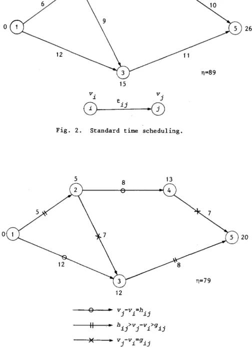
To illustrate our algorithm, consider an arrow diagram shown in Fig. 1. We use a labeling procedure with "first labeled first scanned rule".

Phase 1.

We set t . . =h . . for each (i,j)eA, and get the earliest starting node times,

~J ~J

which are shown in Fig. 2. an optimal solution of p(O)

As v

S-v1=26>20=PO' we shorten vS-v1 to PO' and get

in Fig. 3. Phase 2.

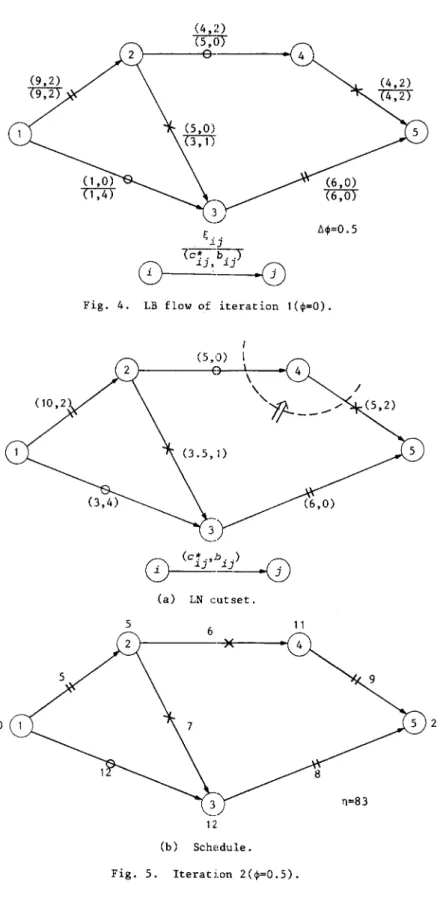
Iteration 1. We determine a .. and B . . for (v,t) in Fig. 3. In Fig. 4, for

~J ~J

each branch (i,j), (c~., b .. ) and its conditipn (the range of v.-v.) are shown.

~J ~J ] ~

(Refer to Fig. 3 for meanings of branch symbols.) We can know a .. and 8 .. by

~J ~J

them. For example, for (1,2), a

12=812=(9,2) as h12>v2-v1>g12. For (1,3),

a

13=(1,4) and 813=(0,0) as v3-v1=h13•

Since there exists an LB flow, which is the L-max flow at termination of phase

1, we go to step 2. A1 is empty, A₂={(2,3),(2,4)}, and

~~ = min(-(3-S)/(1-0), -(S-4)/(0-2») = O.S.

Therefore, ~ is increased to O.S.

Iteration 2. See Fig. S. There exists an LN cutset. N_O={1,2,3,S}, and

y=(0,-2). Cl is empty, C₂={(2,4)} and C

3={(4,S)}. Hence, and ~v = min(13-S-6, 10-20+13) = 2, v 4 = 13-2 11, t24

=

8-2

=

6,

n

=

79+2x2

=

83.

The new schedule is shown in Fig. S(b).

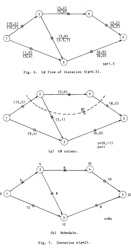
Iteration 3. See Fig. 6. There exist an LB flow. A1 is empty, A₂={(2,3)},

~~ = -(3.S-S)/(1-0) = 1.S,

~ = 0.5+1.5 = 2.

Iteration 4. See Fig. 7. There exists an LN cutset. N

O={1,3,5}, and y=(O,-l). Cl is empty, C₂={( 1,2)} and C₃={ (2,3), (~.,5)

L

Iw = min(5-0-4, 9-12+5, 10-20+11) 1. The new schedule is shown in Fig. 7(b).

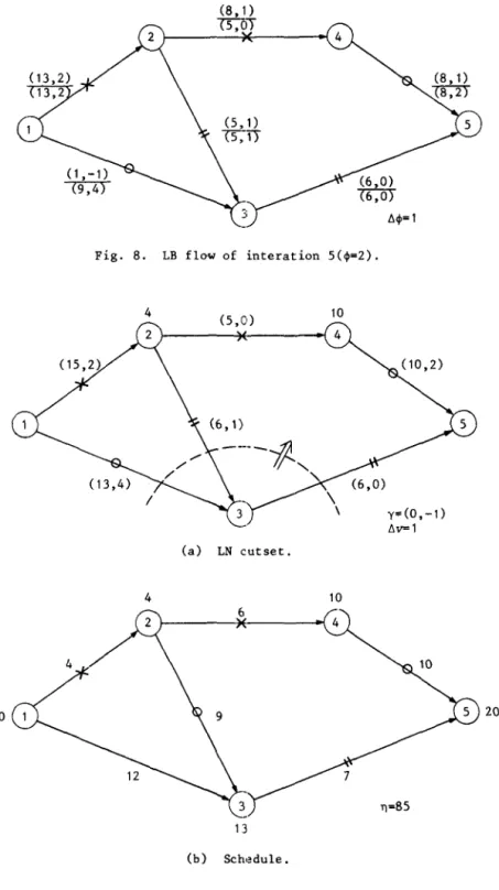
Iteration 5. See Fig. 8. There exists an LB flow. A

1={(1,3)}, and A2 is empty.

~~ = 1, and ~ = 2+1 = 3.

Iteration 6. See Fig. 9. There exists an LN cutset. N_O={3}, and y=(O,-l). Cl is empty, C

2={(3,5)}, and C3={(2,3)}. (Note that (1,3) does not belong to

C₃·)

~v = min(20-12-6, 9-12+4) = 1.

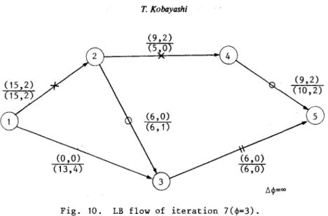
The new schedule is shown in Fig. 9(b). (As 1 belongs to NO' we use (4.6').) Iteration 7. See Fig. 10. There exists an LB flow, but both Al and A2 and are empty. Therefore, ~~=co and we terminate our algorithm.

(6,4)

(9,2)

(8,6) (5,0)

Fig. 1. Arrow diagram.

(10,7) (4.2)

p =20

6 8 14

o

26 15 v. v. ~ t .. ]

CD

~J

-0

Fig. 2. Standard time scheduling.

12

--ttll---

h .. >v .-v .>g ..

~J ] ~ ~J

Fig. 3. An optimal solution of P(O).

o

(9,2) ~ ~----~~---~ 4 (6,0) t6,O) L'l<P=o_s

Fig_ 4. LB flow of iteration 1(~=O).

(5,0)

0

(clj'b i }

·0

(a) LN cutset. 5 6 11 12 (b) Schedule. Fig. 5. Iteration 2(~=0.s).

4

°

t

5 ,2) 5 0) 4

¥s:%

5,2 (5,0) 0.5,1)

Fig. 6. LB flow of iteration 3(~=0.5).

(5,0)

---~/

(a) LN cutset". 4 6 12 (b) Schedule. Fig. 7. Iteration 4(~=2). / . / . / (8,2) y=(O,-l) IIV=1 10

o

(8,1)

n:oT

Fig. 8. LB flow of interation 5(~=2).

4 (5,0) 10 ~---~~---~ 4 (a) LN cutset. 4 10 6 ~---~---~ 4 13 (b) Sch,~dule . Fig. 9. Iteration 6(~=3). (10,2) y=(O,-1) llV=l 10

(9,2) (5,0)

(6,0)

(6,1)

Fig. 10. LB flow of iteration 7(~=3).

Fig. 11 shows the locus of (~,n). For (~,n) on the locus it, there exists an optimal solution of P(~) with n=Ebijt

i j, which is optimal to PO(n). On a horizontal segment, the solution of p(~) does not vary. For a point on a vertical segment, we can obtain a solution of PO(n) by linear interpolation of two solutions of P(~) corresponding to terminal points of the segment.

80

75

o

2 3 4

7. The Case with Negative b's

When some negative b's exist, we must modify our algorithm. Suppose that ck1>0 and bk1<0. Let

cj>kl

=

_{-ck1/bk1 •}

If cj»cj>kl' ck~(cj»<O, and hence tkl is always equal to gkl. «3.5) is not necessarily satisfied.) Therefore, we replace hkl with gkl' and (ck1(cj»,b

k1) with (0,0) at cj>=cj>kl. «k,l) stays in A

p1UAp4 after that.) To stop at cj>=cj>kl' in step 3 of phase 2, replace ~cj> in (4.2) by

where

When two or more negative b's exist, ~cj>3 is defined by i',cj>3

=

min (-c,":(~)/b, ,),

( ' _~,J ') A _{E: 3} ~J ~J wjere

8. Concluding Remark

Our algorithm is also applied to a project scheduling problem with two objectives. Suppose that we wish to minimize

and

z (t)

C LC, ,(h , ~J ~J ,"':t, .) , ~J

Zb(t)

=

Lbij(hij-tij)

subject to (2.1), (2.2) and (2.3). Le't us combine them as

Z(t)

=

zc(t)+cj>ozb(t).

References

[1] Edmonds, L. R., and Karp, R. M.: Theoretical Improvements in Algorithmic

Efficiency for Network Flow Problems. Journal of the Association for

Computing Machinery, Vol.19, No.2 (1972), 248-264.

[2] Ford, L. R., Jr., and Fulkerson, D. R.: Flows in Networks. Princeton

University Press, Princeton, New Jersey, 1962.

[3] Imai, H.: On the Practical Efficiency of Various Maximum Flow Algorithms.

Journal of the Operation Research Society of Japan, Vol.26, No.1 (1983), 61-82.

[4] Iri, M.: Network Flow, Transportation and Scheduling: Theory and

Algo-rithms. Academic Press, New York, 1969.

[5] Iri M., and Kobayashi, T.: Network Theory (in Japanese).

Nikkagiren-shuppan, Tokyo, 1976.

[6] Jewell, W. S.: Divisible Activities in Critical Path Analysis.

Opera-tions Research, Vol.13, No.5 (1965), 747-760.

[7] Kelley, J. E., Jr.: Critical Path Planning and Scheduling: Mathematical

Basis. Operations Research, Vol.9, No.2 (1961), 296-320.

[8] Kobayashi, T.: Note on the Critical Path Analysis for a Project with a

Divisible Activity. Journal of the Operations Research Society of Japan,

Vol.9, Nos. 3 & 4 (1967), 137-140.

[9] Kobayashi, T.: Critical Path Analysis for a Project with Divisible

Activities. Journal of the Operations Research Society of Japan, Vol.ll,

No.2 (1968), 55-65.

[10] Kobayashi, T.: The Lexico-Shortest Route Algorithm for Solving the

Minimum Cost Flow Problem with an Additional Linear Constraint. Journal

of the Operations Research Society of Japan, Vol.26, No.3 (1983), 167-184.

[11] Tone, K.: On Optimal Pattern Flows. Journal of the Operations Research

Society of Japan, Val.20, No.2 (1977), 77-93.

Takashi KOBAYASHI: Graduate School for Policy Science, Saitama University, Shimo-okubo, Urawa, Saitama, 338, Japan.