Vol. 54, No. 4, December 2011, pp. 201–218
A NONLINEAR CONTROL POLICY USING KERNEL METHOD FOR DYNAMIC ASSET ALLOCATION
Yuichi Takano Jun-ya Gotoh
Tokyo Institute of Technology Chuo University
(Received July 31, 2011; Revised October 3, 2011)
Abstract We build a computational framework for determining an optimal dynamic asset allocation over multiple periods. To do this, we use a nonlinear control policy, which is a function of past returns of investable assets. By employing a kernel method, the problem of selecting the best control policy from among nonlinear functions can be formulated as a convex quadratic optimization problem. Furthermore, we reduce the problem to a linear optimization problem by employing L1-norm regularization. A numerical experiment was conducted wherein scenarios of the rate of return of investable assets were generated by using a one-period autoregressive model, and the results showed that our investment strategy improves an investment performance more than other strategies from previous studies do.
Keywords: Finance, multi-period portfolio optimization, control policy, kernel method,
conditional value-at-risk
1. Introduction
In this paper, we investigate an optimal policy for investing in financial assets over multiple periods. The importance of the multi-period model for making long-term investments has become widely recognized (e.g., Mulvey et al. [17]). A motivation for using multi-period models rather than single-period models can be found in a fact that the rate of return on an asset is dependent on its time series. For example, DeMiguel et al. [6] recently used a vector autoregressive (VAR) model to capture the time-series dependence of stock returns and found that good out-of-sample performance could be achieved on the basis of the VAR model. Their results encouraged us to use multi-period portfolio optimization models together with an appropriate uncertainty modeling.
The multi-period model was first framed as a stochastic control problem [15, 16, 22] (see Infanger [10] for detailed references). Stochastic control aims to design the optimal control policy (or controller) for managing dynamical systems subject to uncertainty. Although the optimal decision rules for portfolio selection and consumption were established at an early stage in [15, 16, 22], it is very difficult to handle stochastic control problems of a practical size because they are computationally burdensome. Consequently, a number of studies have focused on stochastic programming models in which the optimal portfolios are determined instead of optimizing the control policy for managing a portfolio (see, e.g., [4, 5, 7, 12, 14, 18, 27]). Most of the stochastic programming models employ either a simulated path structure or a scenario tree structure for representing the uncertainty of asset returns (see, e.g., [8, 26]), and these models can be integrated into a hybrid model by Hibiki [9].
The simulated path model describes multi-period scenarios of asset returns using a num-ber of simulated paths. It can be easily calibrated to actual market behavior, but a “non-anticipativity condition” is required in the optimization so as to prevent investment decisions
from depending on future observations on simulated paths. Without this condition, different investment decisions could be made from one scenario to another and, accordingly, could be meaningless.
By contrast, the scenario tree model enables one to make conditional investment decisions in each future state in response to the observations of the history until that state. It has been demonstrated, e.g., in [11, 13], that stock returns are serially dependent; therefore, it is probably effective to dynamically rebalance the portfolio on the basis of the observed realization at the time of the decision. The scenario tree model, however, is disadvantageous in that the size of the optimization problem grows exponentially as the number of time periods increases.
In view of these facts, we shall use a control policy, which is represented as a function of portfolio adjustments, in the simulated path model. Although this policy enables us to make conditional investment decisions in the simulated path model as well as in the scenario tree model, its use generally leads to infinite-dimensional and nonconvex optimization.
One remedy for this drawback is to employ a “sub-optimal” solution, namely, to restrict possible decision rules to the class of control policies that are affine functions of the past outcomes (see, e.g., [1–3, 20, 25]). Although this sub-optimal solution is computationally effective, it is clear that this approach may not make the best control policy.
The purpose of this paper is to build a computational framework for determining an optimal control policy among nonlinear functions for dynamic asset allocation over multiple periods. To the best of our knowledge, no studies have ever tried to find an optimal nonlinear control policy by solving a computationally tractable optimization problem. The multi-period portfolio optimization model we consider has been devised by making reference to [1–3]. However, our model differs from what is presented in those papers in that
▷ our model is a scenario-based stochastic programming model, and thus, we can optimize
the nonlinear control policy by utilizing the kernel method;
▷ we employ the conditional value-at-risk (CVaR), which has desirable properties as a risk
measure (see, e.g., [19, 21]), whereas [1–3] employ the variance as a risk measure.
The kernel method is an engine for dealing with the strong nonlinearity of statistical models in machine learning (see, e.g., [23]). By utilizing the kernel method, we can formulate the simulated path model for finding an optimal control policy among nonlinear functions as a convex quadratic optimization problem. Further, by employing an L1-norm regularization, we can reduce the problem to a linear optimization. In the computational experiments, we first generated scenarios of the rate of return of investable assets by using a one-period autoregressive model along the lines of [6] to take into account the serial dependence of stock returns. We then compared the investment performance of our nonlinear control policy with those of other commonly-used models, i.e., a basic simulated path model and a model using linear control policies.
The rest of the paper is organized as follows: In Section 2, we describe the portfolio dynamics and present the basic simulated path model. In Section 3, we formulate the problem of optimizing a nonlinear control policy by utilizing the kernel method. Numerical results are given in Section 4, and conclusions are drawn in Section 5.
2. Portfolio Dynamics and Basic Optimization Model
After giving a mathematical description of portfolio dynamics, we formulate the basic multi-period portfolio optimization model with a simulated path structure.
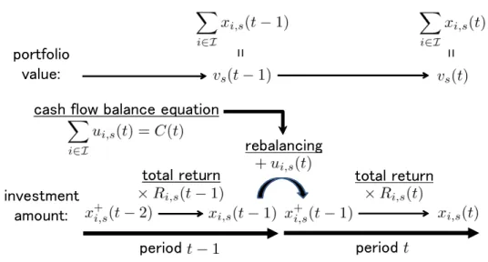
investment amount: period period portfolio value: = =
cash flow balance equation
rebalancing
total return total return
Figure 1: Portfolio dynamics in scenario s
2.1. Preliminaries and portfolio dynamics
The terminology and notation used in this paper are as follows:
Index Sets
I := {1, 2, ..., I} : index set of investable financial assets (where asset 1 is cash)
S := {1, 2, ..., S} : index set of given scenarios (or simulated paths) T := {1, 2, ..., T } : index set of planning time periods
Decision Variables
ui(t) : adjustment of asset i at the beginning of period t (i∈ I, t ∈ T )
ui,s(t) : adjustment of asset i at the beginning of period t under scenario s
(i∈ I, s ∈ S, t ∈ T \ {1})
xi,s(t) : investment amount in asset i at the end of period t under scenario s
(i∈ I, s ∈ S, t ∈ T )
x+i (0) : investment amount in asset i at the beginning of the first period (i∈ I)
x+i,s(t) : investment amount in asset i at the beginning of period t + 1 under scenario s (i∈ I, s ∈ S, t ∈ T \ {T })
vs(t) : portfolio value at the end of period t under scenario s (s∈ S, t ∈ T )
Given Constants
¯
xi(0) : the initial holdings of asset i (i∈ I)
C(t) : net cash flow at the beginning of period t (t∈ T )
Ri,s(t) : total return of asset i in period t under scenario s (i∈ I, s ∈ S, t ∈ T )
Ps : occurrence probability of scenario s (s∈ S) Figure 1 illustrates portfolio dynamics in a scenario s. We assume that there are no transaction costs and that one has an initial portfolio ¯xi(0), i ∈ I. If the investor has no initial endowments, ¯xi(0) are set to 0 for all i∈ I.
One starts investing by adjusting the portfolio as follows:
x+i (0) = ¯xi(0) + ui(1). (2.1) From the definition of the total return of each asset, the investment amount changes over the first period as
Similarly to the first period, we rebalance the portfolio at the beginning of period t ∈
T \ {1}:
x+i,s(t− 1) = xi,s(t− 1) + ui,s(t), (2.3) and the investment amount at the end of period t∈ T \ {1} is as follows:
xi,s(t) = Ri,s(t) x+i,s(t− 1). (2.4) Consequently, the following portfolio dynamics equations are derived from (2.1) through (2.4):
xi,s(1) = Ri,s(1) (¯xi(0) + ui(1)) ,
xi,s(t) = Ri,s(t) (xi,s(t− 1) + ui,s(t)) , t∈ T \ {1}.
(2.5) The portfolio value at the end of period t∈ T in scenario s is the sum of investments:
vs(t) = ∑
i∈I
xi,s(t),
and the expected portfolio value at the end of period t∈ T is ∑s∈SPsvs(t).
In addition, the adjustments must satisfy the following cash flow balance equations in
each period: ∑ i∈I ui(1) = C(1), ∑ i∈I ui,s(t) = C(t), t∈ T \ {1}.
When a self-financing portfolio is considered, the net cash flow C(t) is set to 0 for all t∈ T .
2.2. Basic optimization model
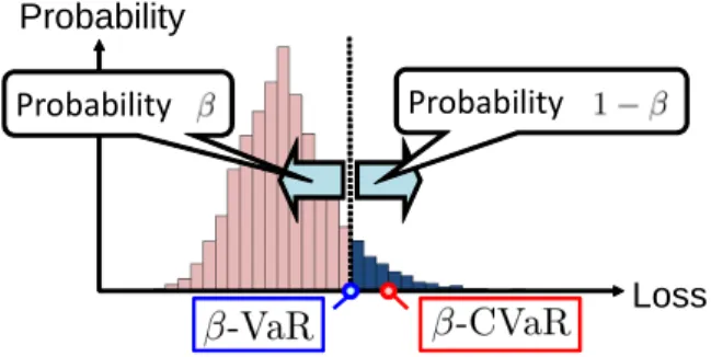
The investment performance of portfolio selection models is usually assessed by using mea-sures of profitability and risk. In this paper, we use the expected portfolio value as a measure of profitability and the conditional value-at-risk (CVaR) as a measure of risk. CVaR has desirable computational and theoretical properties (see, e.g., [19, 21] for the details).
Let β ∈ (0, 1) denote a confidence level. β-CVaR can then be explained as the conditional expectation of a random loss exceeding the β-value-at-risk (β-VaR), which is the β-quantile of the random loss (see Figure 2). Now the random loss is defined as the negative of the portfolio value at the end of period t, i.e., −vs(t), and the corresponding CVaR in each period is the optimal value of the following linear optimization problem (see [21]):
min { a(t) + 1 1− β ∑ s∈S Pszs(t) zs(t)≥ −vs(t)− a(t), zs(t)≥ 0, s ∈ S } ,
where a(t) and zs(t) are decision variables for calculating the CVaR in period t∈ T . To take into account the investment performance in all periods, the following weighted sum of the expected portfolio value is employed as a measure of profitability:
∑ t∈T
η(t)∑
s∈S
Psvs(t), (2.6)
the following weighted sum of CVaR is employed as a measure of risk: ∑ t∈T θ(t) ( a(t) + 1 1− β ∑ s∈S Pszs(t) ) , (2.7)
Probability
Loss Probability
Probability
Figure 2: Value-at-risk and conditional value-at-risk
and the objective function to be minimized is given by the following weighted sum of the measures of profitability and risk:
(1− α)∑ t∈T θ(t) ( a(t) + 1 1− β ∑ s∈S Pszs(t) ) − α∑ t∈T η(t)∑ s∈S Psvs(t), where
η(t) : given nonnegative weight of the expected portfolio value at the end of period t (t∈ T ),
θ(t) : given nonnegative weight of the CVaR at the end of period t (t∈ T ),
α : the trade-off parameter between profitability and risk, α∈ (0, 1).
Moreover, we impose constraints on the investment proportion right after rebalancing:
Li(V + C(1))≤ ¯xi(0) + ui(1) ≤ Ui(V + C(1)) ,
Li(vs(t− 1) + C(t)) ≤ xi,s(t− 1) + ui,s(t)≤ Ui(vs(t− 1) + C(t)) , t ∈ T \ {1}, where V (:= ∑i∈Ix¯i(0)) is the initial wealth, and Li and Ui are lower and upper limits, respectively, of the investment proportion in asset i∈ I. For instance, Li are set to 0 when short-sales are not allowed.
The basic multi-period portfolio optimization model is formulated as a linear optimiza-tion problem: minimize (1− α)∑ t∈T θ(t) ( a(t) + 1 1− β ∑ s∈S Pszs(t) ) − α∑ t∈T η(t)∑ s∈S Psvs(t) · · · (2.8.a) subject to zs(t)≥ −vs(t)− a(t), zs(t)≥ 0, s ∈ S, t ∈ T · · · (2.8.b) xi,s(1) = Ri,s(1) (¯xi(0) + ui(1)) , i∈ I, s ∈ S · · · (2.8.c)
xi,s(t) = Ri,s(t) (xi,s(t− 1) + ui(t)) , i∈ I, s ∈ S, t ∈ T \ {1} · · · (2.8.d)
vs(t) = ∑ i∈I xi,s(t), s∈ S, t ∈ T · · · (2.8.e) ∑ i∈I ui(t) = C(t), t∈ T · · · (2.8.f) Li(V + C(1))≤ ¯xi(0) + ui(1) ≤ Ui(V + C(1)) , i∈ I · · · (2.8.g) Li(vs(t− 1) + C(t)) ≤ xi,s(t− 1) + ui(t)≤ Ui(vs(t− 1) + C(t)) , i∈ I, s ∈ S, t ∈ T \ {1} · · · (2.8.h) (2.8)
with decision variables a(t), ui(t), vs(t), xi,s(t) and zs(t). It should be noted that ui(t) are used in place of ui,s(t) in problem (2.8) in order to satisfy the non-anticipativity condition, which makes the adjustments, ui,s(t), independent of the future total returns, Ri,s(k), k ≥ t.
3. Optimization of Control Policy
3.1. Control policy for making investment decisions
The basic optimization model (2.8) determines the value of adjustments ui(t) for “all” periods t ∈ T at the beginning of the planning horizon. This is clearly disadvantageous because only ui(1) are here-and-now decisions and ui(t), t ∈ T \ {1}, are wait-and-see decisions in the multi-stage stochastic programming model (see, e.g., [24]). That is, only
ui(1) must be fixed at the beginning of the planning horizon, and it is possible to determine
ui(t), t ∈ T \ {1}, on the basis of information available at the end of period t − 1, i.e., on the basis of the actual values of the investment amounts xi,s(k) and the total returns Ri,s(k) for 1 ≤ k ≤ t − 1 (see also Figure 1). By taking advantage of such available information and exploiting the serial dependence of stock returns, we have a chance of improving the investment performance.
We employ a control policy to make conditional investment decisions. The control policy is defined as a function of the past investment amount and the past total return. Specifically, with a control policy Fi,t, the adjustments ui,s(t) are determined as follows:
ui,s(t) =Fi,t(xs(t− 1), Rs(t− 1)) , t ∈ T \ {1}, (3.1) where
xs(t) := (xi,s(k); i∈ I, 1 ≤ k ≤ t) , Rs(t) := (Ri,s(k); i∈ I, 1 ≤ k ≤ t) .
Note that the control policies Fi,t are independent of the scenario s; therefore, using the control policy does not violate the non-anticipativity condition. Additionally, the adjust-ments ui,s(t) depend on the past outcomes xs(t− 1) and Rs(t− 1), and consequently, we can make conditional investment decisions about each scenario.
Next, we show that the past investment amounts, xs(t− 1), can be omitted from the control policy (3.1) by following Calafiore and Campi [3]. To begin with, we derive the following expression by successively using the portfolio dynamics equations (2.5):
xi,s(t) = Ri,s(t) (xi,s(t− 1) + ui,s(t)) = Ri,s(t) xi,s(t− 1) + Ri,s(t) ui,s(t)
= Ri,s(t)Ri,s(t− 1) (xi,s(t− 2) + ui,s(t− 1)) + Ri,s(t) ui,s(t)
= Ri,s(t)Ri,s(t− 1) xi,s(t− 2) + Ri,s(t)Ri,s(t− 1) ui,s(t− 1) + Ri,s(t) ui,s(t) .. . = Gi,s(1, t) (¯xi(0) + ui(1)) + t ∑ k=2 Gi,s(k, t) ui,s(k), (3.2) where
Gi,s(t1, t2) := Ri,s(t1)Ri,s(t1+ 1) · · · Ri,s(t2− 1)Ri,s(t2), t1 ≤ t2.
It follows from (3.1) and (3.2) that
xi,s(t) = Gi,s(1, t) (¯xi(0) + ui(1)) + t ∑ k=2
We can see from this that xi,s(t) can be expressed by xj,s(k), j ∈ I, 1 ≤ k ≤ t − 1, and
Rj,s(k), j ∈ I, 1 ≤ k ≤ t. By performing a similar procedure for xi,s(t− 1), xi,s(t− 2), . . . , we can see that xi,s(t) can be expressed as a function of Rj,s(k), j ∈ I, 1 ≤ k ≤ t, of the form xs(t) =Ht(Rs(t)). It follows that
ui,s(t) =Fi,t(Ht−1(Rs(t− 1)) , Rs(t− 1)) , i ∈ I, s ∈ S, t ∈ T \ {1}.
Since ui,s(t) can be expressed by a function only of Rs(t−1), it is clear that the following control policies have the same ability as the control policies (3.1) to design investment strategies:
ui,s(t) =Fi,t(Rs(t− 1)) , t = T \ {1}. More specifically, we shall consider a control policy of the form,
ui,s(t) = ui(t) + wi(t)⊤ϕi,t(Rs(t− 1)) , t = T \ {1}, (3.3) where ui(t) represent the adjustment actions which are independent of scenarios, and ϕi,t are nonlinear mappings fromRI×(t−1)toRNi,t. After the fashion of machine learning, we call the image of the mapping a feature vector. Note that wi(t) ∈ RNi,t are parameter vectors to be determined and that each element of wi(t) represents the weight of the corresponding feature. A simple example of features would be the following polynomials of degree two:
ϕi,t(Rs(t− 1)) = (Rj,s(k)Rm,s(k) ; j, m∈ I, j ≥ m, 1 ≤ k ≤ t − 1) ,
and Ni,t = I(I + 1)(t− 1)/2. It is clear that high-dimensional feature vector enables one to ensure a greater variety of investment strategies.
3.2. Control policy optimization using the kernel method
We could solve a problem of optimizing the control policy (3.3) after the feature vector functions ϕi,t are properly defined. However, the problem to be solved is intractable if high-dimensional or infinite-dimensional feature vectors are employed.
A reasonable option to overcome this difficulty is restricting the class of control policies to a linear one as is done in [1–3]. The following control policies are linear mappings of the past total returns of µ periods:
ui,s(t) = ui(t)+ t−1 ∑ k=max{t−µ, 1} ∑ j∈I ri,j(k, t) ( Rj,s(k)− ¯Rj(k) ) , i ∈ I, s ∈ S, t ∈ T \{1}, (3.4) where ¯Ri(t) := ∑
s∈SPsRi,s(t). ui(t) represent the nominal adjustment actions, and ri,j(k, t) represent control actions against the past total returns. Both ui(t) and ri,j(k, t) are decision variables for optimizing the control policy.
Note that the control policy (3.4) is not exactly the same as those used in [1–3] because their models are not scenario-based. Although the linear control policy (3.4) leads to a tractable linear optimization problem, nonlinear adjustment actions cannot be implemented. Thus, in this paper, we utilize the kernel method in order to take into account highly nonlinear adjustment actions. The kernel method is a class of algorithm for analyzing nonlinear and complex data in machine learning (see, e.g., [23]). Its greatest merit is that it enables us to estimate an optimal function (3.3) without explicitly computing in a high-dimensional or infinite-high-dimensional feature space. This technique is referred to as the kernel trick in the context of machine learning.
We begin by introducing the regularization terms, ∥wi(t)∥2, i.e., the square of the Eu-clidean norm of wi(t), to our problem. By suppressing the rise in ∥wi(t)∥2, we prevent the control policy from overfitting the total returns Ri,s(t) used in the problem. This is a commonly used approach for enhancing the generalization capability of kernel methods (see, e.g., [23]). By adding regularization terms to the objective, we can consider the following problem of optimizing the control policy (3.3):
minimize (1− α)∑ t∈T θ(t) ( a(t) + 1 1− β ∑ s∈S Pszs(t) ) − α∑ t∈T η(t)∑ s∈S Psvs(t) + λ ∑ i∈I\{1} ∑ t∈T \{1} ∥wi(t)∥2 · · · (3.5.a) subject to zs(t)≥ −vs(t)− a(t), zs(t)≥ 0, s ∈ S, t ∈ T , · · · (3.5.b) xi,s(1) = Ri,s(1) (¯xi(0) + ui(1)) , i∈ I, s ∈ S, · · · (3.5.c)
xi,s(t) = Ri,s(t) (xi,s(t− 1) + ui,s(t)) , i∈ I, s ∈ S, t ∈ T \ {1}, · · · (3.5.d)
vs(t) = ∑ i∈I xi,s(t), s∈ S, t ∈ T , · · · (3.5.e) ∑ i∈I ui(1) = C(1); ∑ i∈I ui,s(t) = C(t), s ∈ S, t ∈ T \ {1}, · · · (3.5.f) Li(V + C(1))≤ ¯xi(0) + ui(1)≤ Ui(V + C(1)) , i ∈ I, · · · (3.5.g) Li(vs(t− 1) + C(t)) ≤ xi,s(t− 1) + ui,s(t)≤ Ui(vs(t− 1) + C(t)) , i∈ I, s ∈ S, t ∈ T \ {1}, · · · (3.5.h) ui,s(t) = ui(t) + wi(t)⊤ϕi,t(Rs(t− 1)) , i ∈ I \ {1}, s ∈ S, t ∈ T \ {1}, · · · (3.5.i) (3.5) with decision variables a(t), ui(t), ui,s(t), vs(t), wi(t), xi,s(t) and zs(t), where λ > 0 is a regu-larization parameter. Note from the constraints (3.5.i) that the control policy is not applied to cash (i = 1). This is because the adjustments of cash, u1,s(t), are uniquely determined
from the adjustments of other assets through the cash flow balance equations (3.5.f). Let
Ki,ℓ,s(t) := ϕi,t(Rℓ(t− 1))⊤ϕi,t(Rs(t− 1)) (3.6) be the kernel function. We prove the following theorem in order to apply the kernel method to the problem (3.5):
Theorem 3.1 (Representer theorem [23]). Let wi∗(t) be optimal solutions to the prob-lem (3.5). Then there are ei,s(t), i∈ I \ {1}, s ∈ S, t ∈ T \ {1} such that
wi∗(t)⊤ϕi,t(Rs(t− 1)) = ∑
ℓ∈S
ei,ℓ(t)Ki,ℓ,s(t), i∈ I \ {1}, s ∈ S, t ∈ T \ {1}.
Proof. Let wi0(t) be a linear combination of feature vectors, ϕi,t(Rℓ(t− 1)), as follows: w0i(t) :=∑
ℓ∈S
Then, by selecting ξi(t) from orthogonal complement of the feature vectors, wi(t) can gen-erally be expressed as follows:
wi(t) = w0i(t) + ξi(t). (3.7) Since all the feature vectors are orthogonal to ξi(t), it follows from (3.7) that
wi(t)⊤ϕi,t(Rs(t− 1)) = wi0(t)⊤ϕi,t(Rs(t− 1)) .
Therefore, we can see from (3.5.i) that the adjustments ui,s(t) are independent of ξi(t). Furthermore, the regularization terms can be expressed as follows:
λ ∑ i∈I\{1} ∑ t∈T \{1} ∥wi(t)∥2 = λ ∑ i∈I\{1} ∑ t∈T \{1} ( ∥w0 i(t)∥ 2+∥ξ i(t)∥2 ) ,
from the orthogonality of w0
i(t) and ξi(t). The minimum of the regularization terms is therefore obtained when ξi(t) = 0, which means that
wi∗(t) = wi0(t) =∑ ℓ∈S
ei,ℓ(t) ϕi,t(Rℓ(t− 1)) . (3.8) This proof is completed by referring to (3.6) and (3.8).
Theorem 3.1 states that the optimal adjustments, u∗i,s(t), can be computed without any concern about the dimensions, Ni,t, of the feature vectors.
Considering that the regularization terms in the problem (3.5) can also be expressed by
λ ∑ i∈I\{1} ∑ t∈T \{1} ∥wi(t)∥2 = λ ∑ i∈I\{1} ∑ t∈T \{1} ∑ ℓ∈S ∑ s∈S
ei,ℓ(t) ei,s(t)Ki,ℓ,s(t) (3.9)
from (3.6) and (3.8), we can see that the problem to be solved can be formulated as a convex quadratic optimization problem (QP):
minimize (1− α)∑ t∈T θ(t) ( a(t) + 1 1− β ∑ s∈S Pszs(t) ) − α∑ t∈T η(t)∑ s∈S Psvs(t) + λ ∑ i∈I\{1} ∑ t∈T \{1} ∑ ℓ∈S ∑ s∈S
ei,ℓ(t) ei,s(t)Ki,ℓ,s(t) · · · (3.10.a) subject to (3.5.b), . . . , (3.5.h), ui,s(t) = ui(t) + ∑ ℓ∈S ei,ℓ(t)Ki,ℓ,s(t), i∈ I \ {1}, s ∈ S, t ∈ T \ {1}, · · · (3.10.b) (3.10) with decision variables a(t), ei,s(t), ui(t), ui,s(t), vs(t), xi,s(t) and zs(t).
Although the problem (3.10) is tractable in the sense that the convex QP is polynomial-time-solvable, it is more beneficial to reduce the problem to a linear optimization problem especially when a large number of financial assets and/or scenarios must be dealt with. Thus, we shall employ an L1-norm regularization of the form,
λ ∑ i∈I\{1} ∑ t∈T \{1} ∑ s∈S |ei,s(t)|, in place of (3.9). In view of the following relation:
problem (3.10) can be reduced to a linear optimization problem (LP): minimize (1− α)∑ t∈T θ(t) ( a(t) + 1 1− β ∑ s∈S Pszs(t) ) − α∑ t∈T η(t)∑ s∈S Psvs(t) + λ ∑ i∈I\{1} ∑ t∈T \{1} ∑ s∈S
(wi,s(t) + yi,s(t)) · · · (3.11.a) subject to (3.5.b), ..., (3.5.h),
wi,s(t)≥ 0, yi,s(t)≥ 0, i ∈ I \ {1}, s ∈ S, t ∈ T \ {1}, · · · (3.11.b)
ui,s(t) = ui(t) + ∑
ℓ∈S
(wi,ℓ(t)− yi,ℓ(t))Ki,ℓ,s(t), i∈ I \ {1}, s ∈ S, t ∈ T \ {1},
· · · (3.11.c)
(3.11) with decision variables a(t), ui(t), ui,s(t), vs(t), wi,s(t), xi,s(t), yi,s(t) and zs(t).
Note that Theorem 3.1 does not apply when the L1-norm is employed in the regular-ization terms. Problem (3.11), however, is clearly an approximation of problem (3.10). We shall verify the practical effectiveness of a solution to problem (3.11) in the next section.
4. Numerical Experiments
The numerical results presented in this section show the investment performance of the kernel control policy, i.e., the control policy obtained by solving the problem (3.11). All computations were conducted on a Windows 7 personal computer with a CORE i5 Processor (2.40GHz) and 4GB memory, and NUOPT (ver. 13.1.5), a mathematical programming software package developed by Mathematical System, Inc., was used to solve the LPs.
We considered five financial assets (i.e., I = 5) over a planning horizon of five periods (i.e., T = 5) and in 200 scenarios (i.e., S = 200). The initial holdings were set as ¯x1(0) := 100
and ¯xi(0) := 0 for i∈ I \{1}. The lower limit, Li, and the upper limit, Ui, of the investment proportion were set to 0 and 0.5, respectively, for all i∈ I. The net cash flow, C(t), was 0 for all t∈ T . The occurrence probability, Ps, was 1/S for all s∈ S and the confidence level,
β, was 0.9. The weights of CVaR, θ(t), and those of the expected portfolio value, η(t), were
set as θ(T ) = η(T ) = 1 and θ(t) = η(t) = 0 for t ∈ T \ {T }. We employed the following Gaussian kernel, which corresponds to an infinite-dimensional feature space, as the kernel function for problem (3.11):
Ki,ℓ,s(t) = exp − ∑ j∈I t∑−1 k=1 (Rj,ℓ(k)− Rj,s(k))2 σ2 i,t ,
We compared the efficiency of the following models and parameter settings:
Basic : the basic optimization model (2.8),
Linear(1) : the optimization model using the linear control policy (3.4) with µ = 1, Linear(4) : the optimization model using the linear control policy (3.4) with µ = 4, Kernel(a,a) : our optimization model (3.11) with λ = 0.00001 and σi,t = 0.1
√ t− 1,
Kernel(a,b) : our optimization model (3.11) with λ = 0.00001 and σi,t = 0.4
√ t− 1,
Kernel(b,a) : our optimization model (3.11) with λ = 0.001 and σi,t = 0.1
√ t− 1,
Kernel(b,b) : our optimization model (3.11) with λ = 0.001 and σi,t = 0.4
√ t− 1. (4.1) 4.1. Scenario generation
DeMiguel et al. [6] showed that the out-of-sample investment performance can be substan-tially improved by exploiting the serial dependence of stock returns. Based on the vector autoregressive (VAR) model in [6], we randomly generated scenarios of the total returns,
Ri,s(t), by using the following one-period autoregressive model of the rate of returns ˜Ri(t)−1,
i∈ I \ {1}: ˜ Ri(t)− 1 = γi+ ∑ j∈I\{1} δi,j ( ˜ Rj(t− 1) − 1 ) + ˜εi(t), i∈ I \ {1},
where γi are intercepts and δi,j are coefficients of the asset j’s rate of return, and ˜εi(t) are random errors. Note that asset 1 was cash and R1,s(t) were set to 1 for all s ∈ S and
t ∈ T , without loss of generality. We assumed that ˜εi(t) are independently and identically distributed with respect to t∈ T .
We collected monthly data of investment fund’s base price from 2003 to 2010 from the Yahoo finance Japan∗. Specifically, asset 2 was a fund investing in large-sized and value stocks, asset 3 was a fund investing in large-sized and growth stocks, asset 4 was a fund investing in small-sized and value stocks, and asset 5 was a fund investing in small-sized and growth stocks.
The estimated values of the parameters γi, i∈ I \ {1}, and δij, i, j ∈ I \ {1}, were 0.0064 0.0035 0.0111 0.0176 and 0.404 0.074 0.108 −0.273 0.338 0.073 0.089 −0.259 0.539 0.022 0.235 −0.427 0.388 0.381 0.152 −0.437 , respectively.
We assumed that ˜εi(t) follow a multivariate normal distribution with zero mean and the
variance-covariance matrix Σ. The estimated value of Σ was as follows: Σ = 0.0026 0.0023 0.0028 0.0030 0.0023 0.0024 0.0027 0.0030 0.0028 0.0027 0.0038 0.0036 0.0030 0.0030 0.0036 0.0048 .
It was found from the values of γi and diagonal elements of Σ that assets 4 and 5, both of which consist of small-sized stocks, are relatively high-risk and high-return.
4.2. Performance evaluation methodology
We generated two different sets of scenarios: a training set {Ri,s(t)| i ∈ I, s ∈ S, t ∈ T } and a testing set{Rout
i,s(t)| i ∈ I, s ∈ Sout, t ∈ T }, where Sout is a set of scenarios of size S and Sout∩ S = ∅. The optimization problems (4.1) are formulated and solved by using the training set. Let us denote the optimal solutions to the problems (4.1) by u∗i(t), ri,j∗ (k, t),
w∗i,s(t) and y∗i,s(t).
The in-sample performance was evaluated on the basis of the training set. The out-of-sample performance was then evaluated as follows: In the case of the basic optimization model (2.8), the performance of the adjustments uout
i (t) = u∗i(t) were evaluated on the basis of the testing set. In the case of the linear control policy (3.4), the out-of-sample performance was evaluated on the basis of the testing set by using the following adjustments:
uouti (1) = u∗i(1), i ∈ I, uouti,s(t) = u∗i(t) + t−1 ∑ k=max{t−µ, 1} ∑ j∈I r∗i,j(k, t)(Routj,s(k)− ¯Rj(k) ) , i∈ I \ {1}, s ∈ Sout, t∈ T \ {1}, uout1,s(t) = C(t)− ∑ i∈I\{1}
uouti,s(t), s∈ Sout, t∈ T \ {1}.
We employed the following Gaussian kernel function in the model (3.11) for the out-of-sample performance evaluation:
Kout i,ℓ,s(t) = exp − ∑ j∈I t∑−1 k=1 ( Rj,ℓ(k)− Routj,s(k) )2 σ2 i,t ,
and then we evaluated the out-of-sample performance on the basis of the testing set by using the following adjustments:
uouti (1) = u∗i(1), i∈ I,
uouti,s(t) = u∗i(t) +∑ ℓ∈S
(
w∗i,ℓ(t)− yi,ℓ∗ (t))Kouti,ℓ,s(t), i∈ I \ {1}, s ∈ Sout, t∈ T \ {1}, uout1,s(t) = C(t)− ∑
i∈I\{1}
-94 -92 -90 -88 -86 -84 -82 -80 -78 -76 -74 100 102 104 106 108 110 112 CV aR
Expected Portfolio Value
Basic Linear(1) Linear(4) Kernel(a,a) Kernel(a,b) Kernel(b,a) Kernel(b,b)
Figure 3: Efficient frontier (in-sample, see also (4.1))
4.3. Efficient frontier
Figures 3 and 4 show the efficient frontiers of the solutions to problems (4.1). In Figures 3 and 4, the horizontal axis and vertical axis are the expected portfolio value (2.6) and CVaR (2.7), respectively. Each plot on a frontier corresponds to a different value of the trade-off parameter, α∈ {0.1, 0.2, 0.3, 0.4, 0.5, 0.6, 0.7, 0.8, 0.9}.
In-Sample Performance.
Figure 3 shows the in-sample performance. It can be seen that the solutions to the basic optimization model (2.8) are dominated by those of other models that use control policies. The linear control policy with µ = 4 performs better than the one with µ = 1. The frontiers of Linear(1) and Linear(4) are similar to those of Kernel(b,b) and Kernel(b,a), respectively. The solutions to Linear(1) and Linear(4) are all dominated by those of Kernel(a,b). Moreover, the solutions to Kernel(a,a) overwhelm all the other solutions.
Out-of-Sample Performance.
Figure 4 shows the out-of-sample performance. It can be seen that the solutions to Kernel(a,a) deteriorate. Since these solutions performed the best in the in-sample tests, this indicates that Kernel(a,a) overfitted the training scenario set. The solutions to the basic optimization model (2.8) are still dominated by those of the models, except Kernel(a,a); however, the differences among them are smaller in the out-of-sample tests than in the in-sample tests. The solutions to Kernel(a,b) dominate those of all the other models when a high-return investment is made. Most of the solutions to Linear(4) are dominated by those of Kernel(a,b), but the difference is not very large. Also, Linear(1) and Kernel(b,b) attain low CVaRs when a low-risk investment is made.
-88 -86 -84 -82 -80 -78 -76 -74 100 101 102 103 104 105 106 107 108 CV aR
Expected Portfolio Value
Basic Linear(1) Linear(4) Kernel(a,a) Kernel(a,b) Kernel(b,a) Kernel(b,b)
Figure 4: Efficient frontier (out-of-sample, see also (4.1))
Table 1: CPU time (in seconds, see also (4.1))
Basic Linear(1) Linear(4) Kernel(a,a) Kernel(a,b) Kernel(b,a) Kernel(b,b)
min 3.1 51.1 90.4 183.9 159.8 198.9 172.1
average 3.4 71.1 107.3 209.1 171.1 216.1 197.3
max 3.7 90.8 138.7 230.2 189.7 230.3 219.7
It is clear from Figures 3 and 4 that dynamic asset allocation under a nonlinear control policy is effective if we can properly set the parameters. In addition, the linear control policy, which is a kind of compromise solution to an intractable optimization problem, is comparable to nonlinear control policies in the out-of-sample tests.
Computational Time.
In drawing an efficient frontier in Figure 3, we solved nine optimization problems, each corresponding to α∈ {0.1, 0.2, 0.3, 0.4, 0.5, 0.6, 0.7, 0.8, 0.9}. Table 1 shows the minimum CPU time (min), the average CPU time (average), and the maximum CPU time (max) of each model. Although our model improved the investment performance, its CPU time to arrive at a solution was longer than those of other models.
4.4. Investment amounts in out-of-sample tests
Figure 5 shows the boxplots of the investment amounts, xi,s(t), in the out-of-sample tests. The boxplot displays the distribution of {xi,s(t) | s ∈ Sout} for each asset i ∈ I and each period t ∈ T . The investment amounts obtained by the basic optimization model (2.8) have a low dispersion relative to those of the linear and kernel control policies. We can interpret this as meaning that the control policies improve the investment performance by
X .1 .1 . X .1 .2 . X .1 .3 . X .1 .4 . X .1 .5 . X .2 .1 . X .2 .2 . X .2 .3 . X .2 .4 . X .2 .5 . X .3 .1 . X .3 .2 . X .3 .3 . X .3 .4 . X .3 .5 . X .4 .1 . X .4 .2 . X .4 .3 . X .4 .4 . X .4 .5 . X .5 .1 . X .5 .2 . X .5 .3 . X .5 .4 . X .5 .5 . -4 0 -2 0 0 2 0 4 0 6 0 8 0 1 0 0 1 1 1 1 1 1 2 3 4 5 Asset : Period : 2 2 2 2 21 2 3 4 53 3 3 3 31 2 3 4 54 4 4 4 41 2 3 4 55 5 5 5 51 2 3 4 5 X.1.1 . X .1 .2 . X .1 .3 . X .1 .4 . X .1 .5 . X .2 .1 . X .2 .2 . X .2 .3 . X .2 .4 . X .2 .5 . X .3 .1 . X .3 .2 . X .3 .3 . X .3 .4 . X .3 .5 . X .4 .1 . X .4 .2 . X .4 .3 . X .4 .4 . X .4 .5 . X .5 .1 . X .5 .2 . X .5 .3 . X .5 .4 . X .5 .5 . -4 0 -2 0 0 2 0 4 0 6 0 8 0 1 0 0 1 1 1 1 1 1 2 3 4 5 Asset : Period : 2 2 2 2 21 2 3 4 53 3 3 3 31 2 3 4 54 4 4 4 41 2 3 4 55 5 5 5 51 2 3 4 5 Basic, α = 0.3 Basic, α = 0.7 X .1 .1 . X .1 .2 . X .1 .3 . X .1 .4 . X .1 .5 . X .2 .1 . X .2 .2 . X .2 .3 . X .2 .4 . X .2 .5 . X .3 .1 . X .3 .2 . X .3 .3 . X .3 .4 . X .3 .5 . X .4 .1 . X .4 .2 . X .4 .3 . X .4 .4 . X .4 .5 . X .5 .1 . X .5 .2 . X .5 .3 . X .5 .4 . X .5 .5 . -4 0 -2 0 0 2 0 4 0 6 0 8 0 1 0 0 1 1 1 1 1 1 2 3 4 5 Asset : Period : 2 2 2 2 21 2 3 4 53 3 3 3 31 2 3 4 54 4 4 4 41 2 3 4 55 5 5 5 51 2 3 4 5 X.1.1 . X .1 .2 . X .1 .3 . X .1 .4 . X .1 .5 . X .2 .1 . X .2 .2 . X .2 .3 . X .2 .4 . X .2 .5 . X .3 .1 . X .3 .2 . X .3 .3 . X .3 .4 . X .3 .5 . X .4 .1 . X .4 .2 . X .4 .3 . X .4 .4 . X .4 .5 . X .5 .1 . X .5 .2 . X .5 .3 . X .5 .4 . X .5 .5 . -4 0 -2 0 0 2 0 4 0 6 0 8 0 1 0 0 1 1 1 1 1 1 2 3 4 5 Asset : Period : 2 2 2 2 21 2 3 4 53 3 3 3 31 2 3 4 54 4 4 4 41 2 3 4 55 5 5 5 51 2 3 4 5 Linear(4), α = 0.3 Linear(4), α = 0.7 X .1 .1 . X .1 .2 . X .1 .3 . X .1 .4 . X .1 .5 . X .2 .1 . X .2 .2 . X .2 .3 . X .2 .4 . X .2 .5 . X .3 .1 . X .3 .2 . X .3 .3 . X .3 .4 . X .3 .5 . X .4 .1 . X .4 .2 . X .4 .3 . X .4 .4 . X .4 .5 . X .5 .1 . X .5 .2 . X .5 .3 . X .5 .4 . X .5 .5 . -4 0 -2 0 0 2 0 4 0 6 0 8 0 1 0 0 1 1 1 1 1 1 2 3 4 5 Asset : Period : 2 2 2 2 21 2 3 4 53 3 3 3 31 2 3 4 54 4 4 4 41 2 3 4 55 5 5 5 51 2 3 4 5 X.1.1 . X .1 .2 . X .1 .3 . X .1 .4 . X .1 .5 . X .2 .1 . X .2 .2 . X .2 .3 . X .2 .4 . X .2 .5 . X .3 .1 . X .3 .2 . X .3 .3 . X .3 .4 . X .3 .5 . X .4 .1 . X .4 .2 . X .4 .3 . X .4 .4 . X .4 .5 . X .5 .1 . X .5 .2 . X .5 .3 . X .5 .4 . X .5 .5 . -4 0 -2 0 0 2 0 4 0 6 0 8 0 1 0 0 1 1 1 1 1 1 2 3 4 5 Asset : Period : 2 2 2 2 21 2 3 4 53 3 3 3 31 2 3 4 54 4 4 4 41 2 3 4 55 5 5 5 51 2 3 4 5 Kernel(a,b), α = 0.3 Kernel(a,b), α = 0.7 Figure 5: Investment amounts in out-of-sample tests (see also (4.1))
enabling flexible investment decisions to be made in each scenario. Although short-sales are not allowed by the constraints on training scenario sets, it can be seen that control policies sometimes sell short in the out-of-sample tests. A rolling-horizon implementation is an effective way to get rid of such a problem. In employing this approach, we periodically solve the multi-period optimization problem and use only the initial adjustments, ui(1), to rebalance the portfolio. As long as we continue to take this approach, we will never sell short (see also the investment amounts in the first period in Figure 5). Even if a rolling horizon is difficult to implement in practice, we think that increasing the number of scenarios in the training set will help prevent control policies from violating constraints in the out-of-sample tests.
It can be seen that when high return is preferred (i.e., α = 0.7), Linear(4) and Kernel(a,b) make large investments in low-return assets (assets 2 and 3) compared with Basic. Similarly, when low risk is preferred (i.e., α = 0.3), Linear(4) and Kernel(a,b) make large investments in high-risk assets (assets 4 and 5) compared with Basic. We can see from these results that the control policy achieves both high return and low risk by efficiently diversifying investments in a wide variety of assets.
5. Conclusions
We built a computational framework to determine an optimal nonlinear control policy for dynamic asset allocation over multiple periods. By utilizing the kernel method, the prob-lem of selecting the best control policy from among nonlinear functions was formulated as a convex quadratic optimization problem. Furthermore, by employing the L1-norm regu-larization, we reduced the problem to a linear optimization problem so that we could solve it reliably and efficiently by using a mathematical programming software package.
We conducted numerical experiments to assess the investment performance of what we call the kernel control policy. Although the CPU time of optimizing the kernel control policy was long compared with other models, our policy resulted in better investment performance than the basic model and linear control policies could give.
A further direction of study is to create a procedure for setting the parameters of the kernel method. Our numerical experiments have shown that the investment performance is highly dependent on the values of the parameters; hence, how to set them is of practical importance. Moreover, there is a real possibility that the actual probability distribution of the total return is much different from what we assumed when determining the control policy. Additional numerical experiments considering such a situation will be reported subsequently.
Acknowledgment
The first author is supported by JSPS Grant-in-Aid for Research Activity Start-up 23810007. The second author is partly supported by MEXT Grant-in-Aid for Young Researchers (B) 23710176.
References
[1] G.C. Calafiore: Multi-period portfolio optimization with linear control policies.
Auto-matica, 44 (2008), 2463–2473.
[2] G.C. Calafiore: An affine control method for optimal dynamic asset allocation with transaction costs. SIAM Journal on Control and Optimization, 48 (2009), 2254–2274. [3] G.C. Calafiore and M.C. Campi: On two-stage portfolio allocation problems with affine
recourse. Proceedings of the Joint 44th IEEE Conference on Decision and Control and
European Control Conference (2005).
[4] D.R. Cari˜no, T. Kent, D.H. Myers, C. Stacy, M. Sylvanus, A.L. Turner, K. Watanabe, and W.T. Ziemba: The Russell-Yasuda Kasai model: An asset/liability model for a Japanese insurance company using multistage stochastic programming. Interfaces, 24 (1994), 29–49.
[5] G.B. Dantzig and G. Infanger: Multi-stage stochastic linear programs for portfolio optimization. Annals of Operations Research, 45 (1993), 59–76.
[6] V. DeMiguel, F.J. Nogales, and R. Uppal: Stock return serial dependence and out-of-sample portfolio performance. AFA 2011 Denver Meetings Paper (2010).
[7] S.-E. Fleten, K. Høyland, and S.W. Wallace: The performance of stochastic dynamic and fixed mix portfolio models. European Journal of Operational Research, 140 (2002), 37–49.
[8] N. Hibiki: Multi-period stochastic programming models using simulated paths for strategic asset allocation. Journal of the Operations Research Society of Japan, 44 (2001), 169–193 (in Japanese).
[9] N. Hibiki: A hybrid simulation/tree stochastic optimization model for dynamic asset allocation. In B. Scherer (ed.): Asset and Liability Management Tools: A Handbook for
Best Practice (Risk Books, London, 2003), 269–294.
[10] G. Infanger: Dynamic asset allocation strategies using a stochastic dynamic program-ming approach. In S.A. Zenios and W.T. Ziemba (eds.): Handbook of Asset and Liability
Management (Elsevier, Amsterdam, 2006), 199–251.
[11] N. Jegadeesh and S. Titman: Returns to buying winners and selling losers: Implications for stock market efficiency. Journal of Finance, 48 (1993), 65–91.
[12] M.I. Kusy and W.T. Ziemba: A bank asset and liability management model. Operations
Research, 34 (1986), 356–376.
[13] A. Lo and A.C. MacKinlay: When are contrarian profits due to stock market overre-action?. The Review of Financial Studies, 3 (1990), 175–205.
[14] C.D. Maranas, I.P. Androulakis, C.A. Floudas, A.J. Berger, and J.M. Mulvey: Solving long-term financial planning problems via global optimization. Journal of Economic
Dynamics & Control, 21 (1997), 1405–1425.
[15] R.C. Merton: Lifetime portfolio selection under uncertainty: The continuous-time case.
Review of Economics and Statistics, 51 (1969), 247–257.
[16] R.C. Merton: Optimum consumption and portfolio rules in a continuous-time model.
Journal of Economic Theory, 3 (1971), 373–413.
[17] J.M. Mulvey, W.R. Pauling, and R.E. Madey: Advantages of multiperiod portfolio models. The Journal of Portfolio Management, 29 (2003), 35–45.
[18] J.M. Mulvey and H. Vladimirou: Stochastic network optimization models for invest-ment planning. Annals of Operations Research, 20 (1989), 187–217.
[19] G.Ch. Pflug: Some remarks on the value-at-risk and the conditional value-at-risk. In S. Uryasev (ed.): Probabilistic Constrained Optimization: Methodology and applications (Kluwer Academic Publishers, Dordrecht, 2000), 272–281.
[20] J.A. Primbs and C.H. Sung: A stochastic receding horizon control approach to con-strained index tracking. Asia-Pacific Financial Markets, 15 (2008), 3–24.
[21] R.T. Rockafellar and S. Uryasev: Conditional value-at-risk for general loss distributions.
Journal of Banking & Finance, 26 (2002), 1443–1471.
[22] P.A. Samuelson: Lifetime portfolio selection by dynamic stochastic programming.
Re-view of Economics and Statistics, 51 (1969), 239–246.
[23] B. Sch¨olkopf and A.J. Smola: Learning with Kernels: Support Vector Machines,
Regu-larization, Optimization, and Beyond (MIT Press, 2001).
[24] A. Shapiro, D. Dentcheva, and A. Ruszczy´nski: Lectures on Stochastic Programming:
Modeling and Theory (SIAM, Philadelphia, 2009).
[25] J. Skaf and S. Boyd: Multi-period portfolio optimization with constraints and transac-tion costs. Working Paper, Stanford University (2008).
[26] M.C. Steinbach: Markowitz revisited: Mean-variance models in financial portfolio anal-ysis. SIAM Review, 43 (2001), 31–85.
[27] Y. Takano and J. Gotoh: Constant rebalanced portfolio optimization under nonlinear transaction costs. Asia-Pacific Financial Markets, 18 (2011), 191–211.
Yuichi Takano
Department of Industrial Engineering and Management Graduate School of Decision Science and Technology Tokyo Institute of Technology
2-12-1-W9-77 Ookayama, Meguro-ku Tokyo 152-8552, Japan