Constant Time Generation of Trees with Degree Bounds

全文

(1)Vol.2010-AL-131 No.8 2010/9/22 IPSJ SIG Technical Report. time. Enumeration of restricted graphs or graphs with configurations has many applications in various fields such as machine learning and chemoinformatics. Enumeration of trees and outerplanar graphs can be used for many purposes including the inference of structures of chemical compounds2),4) . For example, the alkane molecular family {Cn H2n+2 | n ≥ 1} is one of the most fundamental classes of tree-like compounds, where each alkane contains only single bonds (either C-C or C-H bonds). Aringhieri et al.1) designed an algorithm that generates all alkane isomers for a given n in O(n4 )-time delay on average. Our research group has been developing algorithms for enumerating chemical graphs that satisfy given various constraints2)–4) . We have designed efficient branch-and-bound algorithms for enumerating tree-like chemical graphs2),4) , which are based on the tree enumeration algorithm6) , and implementations of these algorithms are available on our web server⋆1 . Our algorithms can enumerate all alkane isomer in O(n2 )-time delay on average2) , improving the O(n4 )-time delay1) . Several algorithms to generate all trees with n vertices without repetition have been already known. The best algorithm9) runs in time proportional to the number of trees, i.e., the time delay is O(1) on average. Nakano and Uno7) gave an O(1)-time delay algorithm to generate all trees with exactly n vertices and diameter d without repetition. However, for applications to chemical graph enumerations, we wish to use an efficient algorithm to generate trees with bounded degrees, because each vertex corresponding to an atom in a chemical graph has a small and fixed degree. In this paper, given a number n of vertices, a lower bound d on the diameter, and a capacity function ∆(k) ≥ 2, k = 0, 1, . . . , ⌊n/2⌋, we consider the problem of enumerating all unrooted trees T with exactly n vertices and a diameter at least d such that the degree of each vertex with distance k from the center of T is at most ∆(k). We give an algorithm that generates all such trees without duplication in O(1)-time delay per output in the worst case using O(n) space. For example, alkane isomers Cn H2n+2 can be regarded as unrooted trees with exactly. Constant Time Generation of Trees with Degree Bounds Bingbing Zhuang†1 and Hiroshi Nagamochi†1 Given a number n of vertices, a lower bound d on the diameter, and a capacity function ∆(k) ≥ 2, k = 0, 1, . . . , ⌊n/2⌋, we consider the problem of enumerating all unrooted trees T with exactly n vertices and a diameter at least d such that the degree of each vertex with distance k from the center of T is at most ∆(k). We give an algorithm that generates all such trees without duplication in O(1)time delay per output in the worst case using O(n) space.. 1. Introduction The problem of enumerating (i.e., listing) all graphs with bounded size is one of the most fundamental issues in graph theory. Time delay of an enumeration algorithm is a time bound between two consecutive outputs. Enumerating graphs with a polynomial time delay would be rather easy since we can examine the whole structure of the current graph anytime. However, algorithms with a constant time delay in the worst case is a hard target to achieve without a full understanding of the graphs to be enumerated, since not only the difference between two consecutive outputs is required to be O(1), but also any operation for examining symmetry and identifying the edges/vertices to be modified to get the next output needs to be executable in O(1) time. One of the common ideas behind efficient enumeration algorithms (e.g.,5),6),8) ) is to define a unique representation for each graph in a graph class as its “parent,” which induces a rooted tree that connects all graphs in the class, called the family tree F, where each node in F corresponds to a graph in the class. Then all graphs in the class will be enumerated one by one according to the depth-first traversal of the family tree F. However, the crucial point to attain an O(1)-time delay is to find a “good” parent which enables us to generate each of the children from a graph in O(1) †1 Graduate School of Informatics, Kyoto University. ⋆1 http://sunflower.kuicr.kyoto-u.ac.jp/tools/enumol/. 1. c 2010 Information Processing Society of Japan ⃝.

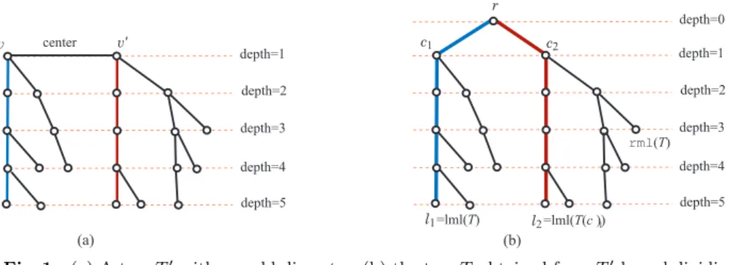
(2) Vol.2010-AL-131 No.8 2010/9/22 IPSJ SIG Technical Report. n carbon atoms (neglecting hydrogen atoms) such that the degree of each vertex is at most four. Hence our result implies that all alkane isomers Cn H2n+2 can be generated in O(1)-time delay in the worst case without duplication, which is an improvement over the O(n2 )-time delay on average2) .. unrooted tree T is called ∆-bounded if 2 ≤ deg(r; T ) ≤ ∆(0) and deg(v; T ) ≤ ∆(dep(v; T )) ∀ v ∈ V (T )−{r}. (1) In this paper, we show the following result. Theorem 1 For an integers n ≥ 3 and d ≤ n, and a capacity function ∆ : [0, ⌊n/2⌋] → [2, n − 1], all ∆-bounded unrooted trees with exactly n vertices and a diameter at least d can be generated in O(1)-time delay in the worst case using O(n) space after an O(n)-time initialization. Let Todd (n, ∆) (resp., Teven (n, ∆)) denote the set of all ∆-bounded unrooted trees with exactly n vertices and an odd (resp., even) diameter.. 2. Preliminaries For two sequences A and B over a set of elements for which a total order is defined, let A > B mean that A is lexicographically larger then B, and let A ≥ B mean that A > B or A = B. Let A = B mean that B is a prefix of A and A ̸= B, and let A ≫ B mean that A > B but B is not a prefix of A. Let A ⊒ B mean that A = B or A = B, i.e., B is a prefix of A. A graph stands for a simple undirected graph, which is denoted by a pair G = (V, E) of a vertex set V and an edge set E. The set of vertices and the set of edges of a given graph G are denoted by V (G) and E(G), respectively. The degree deg(v; G) of a vertex v in a graph G is the number of neighbours of v in G. A path is a sequence of distinct vertices (v0 , v1 , . . . , vk ) such that (vi−1 , vi ) is an edge for i = 1, 2, . . . , k. The length of a path is the number of edges in the path. The distance between a pair of vertices u and v is the minimum length of a path between u and v. The diameter of G is the maximum distance between two vertices in G.. r depth=0. v. v‘. center. depth=1. c1. c2. depth=1 depth=2. depth=2. depth=3. depth=3 rml(T). depth=4. depth=4. depth=5. depth=5. l1 =lml(T). (a). Fig. 1. Unrooted Trees A tree (unrooted tree) is a connected graph without cycles. For two vertices u and v in a tree, let PT (u, v) be the unique path that connects u and v in T . In an unrooted tree, there are at most two vertices the maximum distance from which to other vertices is minimized. If such a vertex v is unique (i.e., the diameter of T is even), then we call v the center of T , and define the depth of a vertex u to be the distance from u to the center. On the other hand, if there are two such vertices v and v ′ (i.e., the diameter of T is odd), then we call the (v, v ′ ) the center of T , and define the depth dep(u; T ) of a vertex u to be the distance from u to the endvertices of the center, i.e., the length of the path from u to the center (v, v ′ ) including the edge (v, v ′ ). Let ∆ : [0, ⌊n/2⌋] → [2, n − 1] denote a capacity function, where ∆(k) is an upper bound on the degree of a vertex v with depth k in an unrooted tree. An. l2 =lml(T(c ))1. (b). (a) A tree T ′ with an odd diameter; (b) the tree T obtained from T ′ by subdividing the center (v, v ′ ) with root r.. Unrooted Rooted Trees We represent unrooted trees as “rooted trees.” A rooted tree is a tree with one vertex r designated as its root. If PT (r, v) has exactly k edges then we say that the depth dep(v; T ) of v is k. The parent of v ̸= r is its neighbour on PT (r, v), and the ancestors of v ̸= r are the vertices on PT (r, v). The parent of the root r and the ancestors of r are not defined. We say that if v is the parent of u then u is a child of v, and if v is an ancestor of u then u is a descendant of v. A leaf is a vertex that has no child. Note that PT (r, v) denotes the set of all ancestors of a vertex v in a rooted tree T , where v ∈ PT (r, v). Now we show how to convert the problem of generating unrooted trees in. 2. c 2010 Information Processing Society of Japan ⃝.

(3) Vol.2010-AL-131 No.8 2010/9/22 IPSJ SIG Technical Report. Todd (n, ∆) ∪ Teven (n, ∆) to a problem of generating rooted trees in some classes. Given a capacity function ∆ : [0, ⌊n/2⌋] → [2, n − 1], let us call a rooted tree T ∆-bounded if it satisfies (1). We call an rooted tree T centerized if T has an even diameter and r is the center of T , i.e., there are two children c1 and c2 of the root r such that the subtrees Ti at ci , i = 1, 2 attain dep(T1 ) = dep(T2 ) = dep(T ) − 1. Let RT (n, ∆) + denote the set of all ∆-bounded centerized trees. Let Todd (n, ∆) denote the set of trees obtained from each tree T ∈ Todd (n, ∆) by subdividing the center (v, v ′ ) with a root r (see Fig. 1(a)-(b)). It is a simple matter to see by definition that the next lemma holds. Lemma 2 (i) For a given integer n ≥ 3, Teven (n, ∆) is given by RT (n, ∆). + (ii) For a given integer n ≥ 2, Todd (n, ∆) is given by RT (n + 1, ∆), where ∆(0) = 2. In what follows, we consider only how to generate rooted trees in RT (n, ∆).. of the root r in an o-tree by c1 , c2 , . . . , cp from left to right. Let OT (T ) denote the set of all o-trees obtained from a rooted tree T . 3. Left-heavy Trees Since all o-trees in OT (T ) of the same tree T are isomorphic, we choose a particular o-tree as the representative of T . For this, we use “left-heavy trees”7) . For an o-tree T ′ , we define the depth sequence L(T ′ ) to be L(T ′ ) = [dep(v1 ; T ′ ), dep(v2 ; T ′ ), . . . , dep(vn ; T ′ )]. If L(T ′ ) > L(T ′′ ) for two ordered trees T ′ and T ′′ , then we say that L(T ′ ) is heavier than L(T ′′ ). An o-tree T ′ ∈ OT (T ) of a rooted tree T is called left-heavy tree if L(T ′ ) ≥ L(T ′′ ) holds for all o-trees T ′′ ∈ OT (T ). For two vertices vi and vj , i ≤ j, let Li,j (T ′ ) = [dep(vi ; T ′ ), dep(vi+1 ; T ′ ), . . . , dep(vj ; T ′ )]. It is known that left-heavy trees can be characterized as follows. Lemma 3 7) An o-tree T ′ ∈ OT (T ) is the left-heavy tree of a rooted tree T if and only if, for a non-root vertex v and its immediate right sibling v ′ of v (if any) in an o-tree T ′ , it holds L(T (v)) ≥ L(T (v ′ )). For each rooted tree T , a left-heavy tree in OT (T ) is unique up to the isomorphism with respect to the root. In what follows, we assume that unordered rooted trees are represented by left-heavy trees. By definition of left-heavy trees, we can easily observe that the following inequality on depth also holds. Lemma 4 For a non-root vertex v and its immediate right sibling v ′ of v (if any) in a left-heavy tree T , it holds dep(T (v)) ≥ dep(T (v ′ )). In particular, dep(T (c1 )) = dep(T (c1 )) ≥ · · · ≥ dep(T (cp )) holds for the children c1 , c2 , . . . , cp of the root r in a left-heavy and ceterized tree T . We call a leftheavy and ceterized T distinguished if, for each i = 1, 2, the number of leaves with the maximum depth in T (ci ) is 1 (i.e., no other leaf than lml(T (ci )) attains dep(T (ci ))). We consider how to add a new leaf along the rightmost path PT (r, rml(T )) of a left-heavy tree T so that the resulting o-tree remains left-heavy. This problem has been solved by Uno and Nakano6) . We here use another solution “competitors” proposed in our companion paper10) , since “competitors” are easier to handle the. Ordered Trees Rooted trees are then represented as “ordered trees.” An ordered tree (o-tree, for short) is a rooted tree with a left-to-right ordering specified for the children of each vertex. For an o-tree T and a vertex in T , let T (v) denote the ordered subtree induced from T by the set of v and descendants of v, preserving the left-to-right ordering for the children of each vertex. For an o-tree T ′ , a leaf v in T ′ is called the leftmost (resp., rightmost) leaf if v is a descendant of the leftmost (resp., rightmost) child of any ancestor of v in T ′ . Let lml(T ′ ) (resp., rml(T ′ )) denote the leftmost (resp., rightmost) leaf in an o-tree T ′ . See Fig. 1(b). Let T be an o-tree with n vertices, and (v1 , v2 , . . . , vn ) be the list of the vertices of T in preorder, i.e., vertices are indexed in the order of DFS. For two vertices u = vi and v = vj , we write u >T v if i < j. Consider two vertices u = vi and v = vj , i ≤ j in T . Let [u, v] denote the set of all vertices vi′ with i ≤ i′ ≤ j, and let T [u, v] denote the graph induced from T by the vertex set [u, v]. Also let lca(u, v) denote the least common ancestor of u and v in T . Let lcaL (u, v) denote the child w of lca(u, v) such that w ∈ PT (r, u), where we let lcaL (u, v) = u if lca(u, v) = u. Similarly, lcaR (u, v) denotes the child w′ of lca(u, v) such that w′ ∈ PT (r, u), where we let lcaR (u, v) = v if lca(u, v) = v. We denote the children. 3. c 2010 Information Processing Society of Japan ⃝.

(4) Vol.2010-AL-131 No.8 2010/9/22 IPSJ SIG Technical Report. Lemma 6 10) In a left-heavy tree T , the competitor of vertex vi is correctly obtained in cases (a) and (b), if any, if the competitors of all vertices vt , t < i have been obtained. In case (a), whether lca(vi , vj ) = lca(vi−1 , vj−1 ) or not can be tested without knowing the value of lca(vi , vj ). For this, we use lca(vi−1 , vj−1 ) and lcaR (vi−1 , vj−1 ) as follows: lca(vi , vj ) = lca(vi−1 , vj−1 ) if and only if j < h and dep(vh ; T ) > dep(vi ; T ) for vh = lcaR (vi−1 , vj−1 ). Hence we can determine the competitor of a new vertex v according to cases (a) and (b) in O(1) time per operation of appending a new leaf.. case where some left part of a left-heavy tree may change. For an o-tree T and a vertex u in T , let T + (u, v) denote the o-tree obtained from T by appending a new vertex v at u as the rightmost child of u. A vertex u in a left-heavy tree T is called valid if T +(u, v) remains left-heavy. Let v be a vertex in an o-tree T . For a descendant vi of v in T , we define the pre-sequence ps(v, vi ) of vi to v to be Lk,i−1 (G) = [dep(vk ; T ), dep(vk+1 ; T ), . . . , dep(vi−1 ; T )] for the child vk of v such that vk is an ancestor of vi . For a vertex vi and a vertex vj with j < i incomparable vi , we call vj pre-identical to vi if ps(v, vj ) = ps(v, vi ) holds, and lcaL (vj , vi ) is the immediate right sibling lcaR (vj , vi ) for v = lca(vj , vi )10) . We define the competitor of a vertex vi to be the vertex vj pre-identical to vi which has the smallest index j (< i) among all vertices pre-identical to vi . A vertex vi has no competitor if no vertex vj , j < i is pre-identical to vi . Lemma 5 10) Let T be a left-heavy tree, let u0 , u1 , . . . , uq (= rml(T )) denote the rightmost path of T . Then there is an index h∗ such that a vertex ui is valid if and only if 0 ≤ i ≤ h∗ . Moreover such an index h∗ is determined as follows. (i) uq has no competitor: Then h∗ = q. (ii) uq has a competitor vj : Let vh be the parent of the vertex vj+1 next to vj in T . Then h∗ = dep(vh ; T ). Let us call such a vertex vh∗ the lowest valid ancestor of uq in T . By maintaining vertices {v1 , v2 , . . . , vn } in an array and the current tree T in a linked data structure, we can compute vh∗ from uq in O(1) time. We review how to compute competitors. For each vertex vi , i = 1, 2, . . . , n in this order, we can set the competitor of a vertex vi to be the vertex vj , j < i which satisfies one of the next cases holds, where we also compute lca(vj , vi ) and lcaR (vj , vi ):. 4. Parent-trees of ∆-bounded Left-heavy Trees In this section, we define the “parent-tree” of each left-heavy tree T in the class RT (n, ∆) of ∆-bounded and centerized trees with n vertices, where dep(T ) − 1 = dep(T (c1 )) = dep(T (c2 )) holds. For ease of applications of the properties on left-heavy trees, we also define the “parent-tree” of each left-heavy tree in RT (n−1, ∆)∪RT (n−2, ∆) with respect to n so that the parent-child relationship over these classes forms a family tree F. We will design an algorithm that visits all nodes in family tree F each in O(1)-time. However, we output only trees in RT (n, ∆) during the traversal of F. For the leftmost and second leftmost children c1 and c2 of the root r in a leftheavy tree T , let ℓi , i = 1, 2 denote the leftmost leaf of the subtree T (ci ) rooted at ci . We call each vertex in PT (r, ℓ1 ) ∪ PT (r, ℓ2 ) a core vertex. Let vlast denote the non-core vertex with the largest preporder index in T . For an even n, let Pn−1 denote the o-tree obtained from a path with n − 1 vertices by choosing its center as the root, and let Pn−1 + i be obtained from Pn−1 by adding a new leaf at the ith vertex vi , i ∈ [0, n/2]. Let RT ([n, n − 2], ∆) denote RT (n, ∆) ∪ RT (n − 1, ∆) ∪ RT (n − 2, ∆). For an odd (resp., even) n, we define the parent-tree of a left-heavy tree T ∈ RT ([n, n− 2], ∆)−{Pn } (resp., T ∈ RT ([n, n −2], ∆)−{Pn−1 +i | 0 ≤ i ≤ n/2}) with respect to n as follows. (1) If T ∈ RT (n, ∆) ∪ RT (n − 1, ∆), then the parent-tree P(T ) of T is defined to be the o-tree T − vlast obtained from T by removing vlast . For example, the parent-tree of T1 with n vertices (reps., T2 with n − 1 vertices) is T2 (resp.,. (a) i ≥ 2 and the previous vertex vi−1 of vi has a competitor vj−1 and it holds lca(vj , vi ) = lca(vj−1 , vi−1 ), where dep(vi−1 ; T ) = dep(vj−1 ; T ) holds: Then the competitor of vi is given by vj . We set lca(vj , vi ) := lca(vj−1 , vi−1 ) and lcaR (vj , vi ) := lcaR (vj−1 , vi−1 ). (b) vi has no such previous vertex vi−1 in case (a), and vi has a left sibling vj : Then the competitor of vi is given by vj . We set lca(vj , vi ) to be the parent of vi and lcaR (vj , vi ) := vi .. 4. c 2010 Information Processing Society of Japan ⃝.

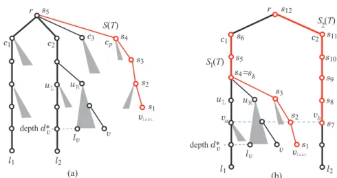
(5) Vol.2010-AL-131 No.8 2010/9/22 IPSJ SIG Technical Report v1 = r. v1 = r. v1 = r. c1. v2. v12. c2. v13. v19. v14. v20. v5. v7. v6 l1 v8. c1. ∆(1)=3. c2. ∆(2)=2. ∆(2)=2. ∆(3)=3. ∆(3)=3. v11. v15 v17 v21 v22. ∆(4)=2. ∆(4)=2. v16 l2. ∆(5)=2. v24. vlast. S2(T). c1. c3. c2. cp. s4. c1. last. l1. l2. l2. S1(T). s2. uR. uL. (c) T3. (b) T2. v. s3. ∆(4)=2 ∆(5)=2. ∆(5)=2. l1. (a) T1. vlast. s1 v1 = r. v1 = r c2. ∆(0)=3. c1. ∆(1)=3. vlast. c2. Fig. 2. l2 (d) T4. depth d*v. ∆(1)=3. ∆(2)=2. ∆(2)=2. ∆(3)=3. ∆(3)=3. ∆(3)=3. ∆(4)=2. ∆(4)=2. ∆(4)=2. ∆(5)=2. ∆(5)=2. l1. vlast vlast. l1. l2 (e) T5. ∆(6)=2. l1. (f) T6. lv l2. (a) Fig. 3. ∆(6)=2. ∆(6)=2. l1. c2. l2. Examples of left-heavy trees for n = 24, where T1 , T4 ∈ RT (n, ∆), T2 , T5 ∈ RT (n − 1, ∆), and T3 , T6 ∈ RT (n − 2, ∆), and Ti+1 is the parent-tree of Ti , i = 1, 2, . . . , 5.. s6. c2 s11. s5. s10. s4 =sk uR. s9 s3. s8 s2. va. ∆(0)=3. c1. ∆(1)=3. ∆(2)=2. ∆(5)=2. uL. vlast. v1 = r. ∆(0)=3. c1. s12. S(T). ∆(1)=3. ∆(3)=3. ∆(2)=2. v10. v4. c2. r. s5. v23. v9. v3. c1. ∆(1)=3. r. ∆(0)=3. ∆(0)=3. ∆(0)=3. v18. vb. s7. v depth d*v. l1. lv. v. (b). s1 vlast l2. (a) Spine S(T ) = {s1 , s2 , . . . , s5 } in a tree T with vlast ̸∈ V (T (c1 )); (b) spine S(T ) = S1 (T ) ∪ S2 (T ) = {s1 , s2 , . . . , s11 } in a tree T with vlast ∈ V (T (c1 )).. tree of T ′ , where T ′ may not be ∆-bounded. A vertex v in T is called unsaturated if deg(v; T ) < ∆(dep(v; T )). In Sections 5.1 and 5.2, we first characterize the set of all child-tree of a left-heavy tree T ∈ RT ([n, n − 2], ∆). In Section 5.3, we next describe an entire algorithm Enumerate for enumerating all left-heavy trees T ∈ RT ([n, n − 2], ∆) by a recursive procedure Gen of generating all childtrees of a given a left-heavy tree T ∈ RT ([n, n − 2], ∆). 5.1 Appending a Leaf to T ∈ RT (n − 1, ∆) ∪ RT (n − 2, ∆) Let T ∈ RT (n − 1, ∆) ∪ RT (n − 2, ∆). By definition of parent-trees, any childtree T ′ of T has n or n − 1 vertices, and T is obtained from T ′ by removing the non-core vertex vlast (T ′ ) with the largest index in T ′ . Thus, T ′ is obtained from T by appending a new leaf (u, v) so that T + (u, v) is left-heavy and ∆-bounded. We here consider when T + (u, v) is left-heavy, i.e., (i) u is a valid vertex in T and (ii) v is the non-core vertex vlast (T + (u, v)) with the largest index in T + (u, v). We define the spine S(T ) of a left-heavy tree T ∈ RT (n − 1, ∆) ∪ RT (n − 2, ∆) as the set of vertices u at which appending a new leaf (u, v) results in an o-tree T + (u, v) such that v is the non-core vertex vlast (T + (u, v)) with the largest index in T + (u, v). By definition of S(T ), we observe the next.. T3 ) in Fig. 2. The inequalities in Lemma 3 still hold in T − vlast , and hence P(T ) = T − vlast remains left-heavy. Clearly P(T ) = T − vlast remains ∆bounded. (2) If T ∈ RT (n − 2, ∆), then the parent-tree P(T ) of T is defined to be the o-tree obtained from T by appending a new leaf to ℓi for each i = 1, 2. For example, the parent-tree of T3 with n − 2 vertices is T4 in Fig. 2. The inequalities in Lemma 3 still hold in P(T ) = (T + (ℓ1 , v)) + (ℓ2 , v ′ ), since the leftmost paths in T (c1 ) and T (c2 ) extend. T − vlast remains left-heavy. Also P(T ) = (T + (ℓ1 , v)) + (ℓ2 , v ′ ) remains ∆-bounded by ∆(dep(ℓ1 ; T )) = ∆(dep(ℓ2 ; T )) ≥ 2. Lemma 7 For each left-heavy tree T ∈ RT ([n, n−2], ∆)−({Pn }∪{Pn−1 +i | 0 ≤ i ≤ n/2}), the parent-tree P(T ) with respect to n is a ∆-bounded left-heavy tree which belongs to RT ([n, n − 2], ∆). 5. Generating Child-trees A left-heavy tree T ′ is called a child-tree of a left-heavy tree T if T is the parent-. 5. c 2010 Information Processing Society of Japan ⃝.

(6) Vol.2010-AL-131 No.8 2010/9/22 IPSJ SIG Technical Report. Lemma 9 Let T ∈ RT (n, ∆) be a distinguished left-heavy tree. If T ′ = T − {ℓ1 , ℓ2 } remains distinguished, then T ′ is left-heavy. We next show how to check whether T can have a non-distinguished child-tree, i.e., whether the o-tree T −{ℓ1 , ℓ2 } remains left-heavy or not. Let X1 = V (T )−{r} and X2 = V (T ) − (V (T (c1 ) ∪ {r}). For each vertex v ∈ Xi , i = 1, 2, we define statei (v) as follows. We first define state1 (v), v ∈ X1 . For the leftmost leaf ℓ1 = lml(T (c1 )) of T (c1 ) and a vertex v ∈ X1 , let us denote uL = lcaL (ℓ1 , v) and uR = lcaR (ℓ1 , v) (see Fig. 3(b)). We compare subtree T (uL ) at uL and subtree TvR = T [uR , v] in the following way. The depth dep(TvR ) of TvR is determined by its leftmost leaf ℓv = lml(TvR ). Hence the depth d∗v = dep(ℓv ; T ) of ℓv in T is given by d∗v = dep(lca(ℓ1 , v); T ) + dep(TvR ) + 1. If T (c1 ) has a non-core vertex u′ <T ℓv with dep(u′ ; T ) > d∗v or uR is not the second leftmost child of lca(ℓ1 , v), then we let state1 (v) = ∅. Then the set of vertices u′ <T ℓv with dep(u′ ; T ) > d∗v consists of core vertices in T (c1 ); i.e., it is given by {u′ ∈ PT (r, ℓ1 ) | dep(u′ ; T ) > d∗v }. Let L∗ be the sequence of depth of the vertices in {u′ ∈ PT (r, ℓ1 ) | dep(u′ ; T ) > d∗v }, and L(T (uL )) − L∗ denote the sequence obtained from L(TvL ) by eliminating the entries in L∗ . We compare the label sequences L(T (uL )) − L∗ and L(TvR ), and define  ∗ ∗ R   (dv , ⊒) if L(T (uL )) − L ⊒ L(Tv ) (2) state1 (v) = (d∗v , ≫) if L(T (uL )) − L∗ ≫ L(TvR )   (d∗ , <) if L(T (u )) − L∗ < L(T R ). L v v. Lemma 8 For each left-heavy tree T ∈ RT (n − 1, ∆) ∪ RT (n − 2, ∆), the o-tree T ′ obtained by appending a new leaf (u, v) is a child-tree of T if and only if u is a valid vertex in S(T ). We show how to find all valid vertices in S(T ) in the following two cases. Case-1: The non-core vertex vlast with the largest index in T does not belong to the subtree T (c1 ): In this case, S(T ) = (s1 = vlast , s2 , . . . , sm = r) is given as the path from the last non-core vertex vlast to the root r. See Fig. 3(a). Since S(T ) is the rightmost path of T , all valid vertices in S(T ) can be identified by the lowest valid ancestor vh∗ = si (1 ≤ i ≤ m) of vlast , and vh∗ can be computed in O(1) time in the same manner in Lemma 5 using the competitor of vlast . Case-2: vlast belongs to the subtree T (c1 ) (i.e., r has only two children and the subtree T (c2 ) is a path): Let va denote the lowest core vertex in T (c1 ) with deg(va ) ≥ 3, and let vb be the vertex vb in T (c2 ) with dep(vb ; T ) = dep(va ; T ). See Fig. 3(b). Then S(T ) consists of two sequences S1 (T ) and S2 (T ), where S1 (T ) = (s1 = vlast , s2 , . . . , st = c1 ) is obtained by visiting the path PT (vlast , c1 ) from vlast to c1 , and S2 (T ) = (st+1 = vb , st+2 , . . . , sm = r) by visiting PT (vb , r) from vb to r, where S1 (T ) is followed by S2 (T ) in S(T ). We easily see that all vertices in S2 (T ) are always valid. For the vertex sk = lca(ℓ1 , vlast ), all vertices sk , sk+1 , . . . , st ∈ S1 (T ) are also valid. The valid vertices in {s1 , s2 , . . . , sk−1 } can be determined by applying Lemma 5 to the subtree T (sK ). Thus the lowest valid ancestor vh∗ = si (1 ≤ i ≤ k − 1) of vlast in T (sK ) can be computed in O(1) time in the same way using the competitor of vlast . Let spn(v) denote the parent v ′ = si+1 ∈ S(T ) of a vertex v = si ∈ S(T ), where spn(r) = ∅. 5.2 Shortening Depth of T ∈ RT (n, ∆) Let T ∈ RT (n, ∆) be a left-heavy tree. By definition of parent-trees, T has at most one child-tree, which is given by T − {ℓ1 , ℓ2 }. Note that T − {ℓ1 , ℓ2 } can be a child-tree of T only when T is distinguished, since the parent-tree of any tree T ∈ RT (n − 2, ∆) with respect to n is distinguished. In fact, for a distinguished left-heavy tree T ∈ RT (n, ∆), T − {ℓ1 , ℓ2 } is a child-tree of T if and only if T − {ℓ1 , ℓ2 } is left-heavy. We show how to examine the left-heaviness of T − {ℓ1 , ℓ2 } in O(1) time. By definition, we first observe the following case.. We define state2 (v), v ∈ X2 analogously with state1 (see Fig. 3(a)). For ℓ2 = lml(T (c2 )) and a vertex v ∈ X2 , let us denote uL = lcaL (ℓ2 , v) and uR = lcaR (ℓ2 , v). Let TvR = T [uR , v] and d∗v = dep(lca(ℓ2 , v); T ) + dep(TvR ) + 1. If T (c2 ) has a noncore vertex u′ <T ℓv with dep(u′ ; T ) > d∗v or uR is not the second leftmost child of lca(ℓ2 , v), then we let state2 (v) = ∅. Otherwise define state2 (v) by (2). Lemma 10 Let T ∈ RT (n, ∆) be a distinguished left-heavy tree such that T ′ = T − {ℓ1 , ℓ2 } is not distinguished. Let d˜ be the current depth dep(ℓ1 ; T ) = dep(ℓ2 ; T ) of T (c1 ) and T (c2 ). Then T − {ℓ1 , ℓ2 } is left-heavy if and only if, for each i = 1, 2, T (ci ) has no non-core vertex v such that statei (v) = (d˜ − 1, <). When a child-tree T is generated from T by appending a new vertex vlast. 6. c 2010 Information Processing Society of Japan ⃝.

(7) Vol.2010-AL-131 No.8 2010/9/22 IPSJ SIG Technical Report. to vˆ in the current tree T ′ , statei , i = 1, 2 are updated as follows. Let the preorder index of vlast in T be K, i.e., vlast = vK . If vK = lml(T (ci )), then statei (vK ) := (dep(vK ; T ), ⊒). Assume vK ̸= lml(T (ci )). If the second term in statei (vK−1 ) is “≫” or “<,” then statei (vK ) := statei (vK−1 ). Assume statei (vK−1 ) = (d∗ , ⊒). Let va = lca(ℓ1 , vK ), and h be the integer such that vK appears as the hth vertex in TvRK . If vertex va+h+1 belongs to TvRK , then set statei (vK ) to be (d∗ , <). Otherwise, we set statei (vK ) to be (d∗ , ≫) (resp., (d∗ , ⊒) and (d∗ , <)) if dep(va+h+1 ; T ) > dep(vK ; T ) (resp., dep(va+h+1 ; T ) = dep(vK ; T ) and dep(va+h+1 ; T ) < dep(vK ; T )).. a diameter at least d. if n is odd then let T be path Pn rooted at its center; Initialize (T); Gen(T ) else /* n is even */ Let Pn−1 be rooted at its center, where (v1 = r, v2 , . . . , vn/2 = ℓ1 ) denotes the path from ℓ1 = lml(Pn−1 ) to the root r; for each unsaturated vi (i.e., vi with ∆(i − 1) ≥ 3) do Let T := Pn−1 +(vi , v) be the tree obtained from Pn−1 by adding a new leaf (vi , v) at vi ; Initialize (T); Gen(T ) endfor endif. When we remove ℓ1 and ℓ2 in the current tree T ′ ∈ RT (n, ∆) and add a new non-core vertex to obtain a child-tree T = T ′ − {ℓ1 , ℓ2 }, we need to recompute the competitor of the current last non-core vertex vlast if T − {ℓ1 , ℓ2 } is not distinguished. Only in this case, vlast ∈ X1 (resp., vlast ∈ X2 ) may have a pre-identical vertex in the subtree T (c1 ) (resp., T (c2 )) of T = T ′ − {ℓ1 , ℓ2 }. We can test whether vlast has a pre-identical vertex in such a subtree T (ci ) or not by checking statei (vlast ). Let dˆ = dep(T ). ˆ ⊒), then set the competitor of vlast to be (i) vlast ∈ X1 : If state1 (vlast ) = (d, the vertex vk′ in T (c1 ) corresponding to vlast , i.e., lca(ℓ1 , vlast ) is a core vertex in T (c1 ) and vk′ is the |V (T (lcaR (ℓ1 , vlast )))|th vertex in subtree T (lcaL (ℓ1 , vlast )). ˆ ⊒), then set the competitor of vlast to be (ii) vlast ∈ X2 : If state2 (vlast ) = (d, the vertex vk′ in T (c2 ) corresponding to vlast , i.e., lca(ℓ2 , vlast ) is a core vertex in T (c2 ) and vk′ is the |V (T (lcaR (ℓ2 , vlast )))|th vertex in subtree T (lcaL (ℓ2 , vlast )). 5.3 Entire Algorithm We are ready to describe the entire algorithm except for showing how to efficiently find unsaturated vertices in the spine S(T ). Algorithm Enumerate constructs initial ∆-bounded left-heavy trees T := Pn for an odd n and T := Pn−1 +i, i ∈ [0, n/2] for an even n before it invokes a recursive procedure Gen of generating child-trees. Algorithm Enumerate(n, ∆, d) Input: An integer n ≥ 3, a capacity function ∆ : [0, ⌊n/2⌋] → [2, n − 1], and an integer d ≤ n. Output: All ∆-bounded left-heavy trees with exactly n vertices and. The above initialization takes O(n) time. The next procedure Gen generates the child-trees T ′ of the current ∆-bounded left-heavy T , and calls Gen(T ′ ) to enumerate all descendants of T ′ . We output only trees T with exactly n vertices at every third depth 3a + 1 of recursive call at T during an execution of Gen. To attain an O(1)-time delay in the worst case, a generated tree T ∈ RT (n, ∆) is output immediately before or after Gen(T ) is executed if a is even (resp., odd). Procedure Gen(T ) Input: A left-heavy tree T ∈ RT ([n, n − 2], ∆). Output: All descendants T ′′ of T such that T ′′ is ∆-bounded left-heavy trees with exactly n vertices and a diameter at least d. if |V (T )| = n and the current depth of recursive calls is 3a + 1 for an even integer a then Output T endif; if |V (T )| = n, T is distinguished, dep(T ) ≥ d + 1, and T − {ℓ1 , ℓ2 } is left-heavy then T ′ := T − {ℓ1 , ℓ2 }; Gen(T ′ ) endif; if |V (T )| = n − 2orn − 1 then for each unsaturated and valid vertex u in S(T ) do Let T ′ := T + (u, v) be obtained from T by adding a new leaf (u, v) ; at u; Gen(T ′ ). 7. c 2010 Information Processing Society of Japan ⃝.

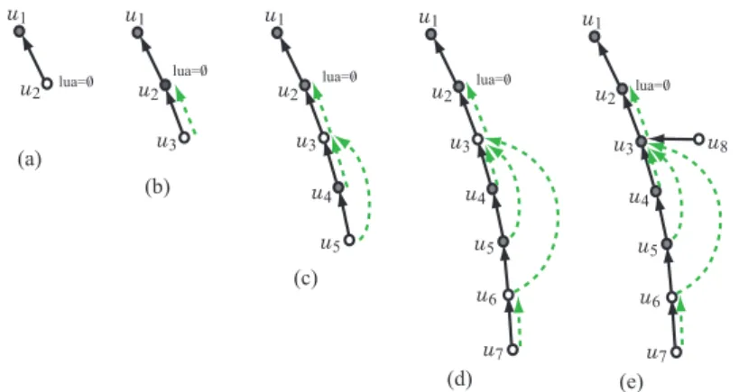
(8) Vol.2010-AL-131 No.8 2010/9/22 IPSJ SIG Technical Report. valid by Lemma 5. When a child-tree T ′ is generated from T by appending a new vertex v to vˆ, we need to update spn and lua (see Fig. 4), where lua(v) never changes since it is only updated once when v is newly added to the tree. Including the maintenance of all data values, we can find all unsaturated and valid vertices in the spine S(T ) in O(1) time per each, where we omit the detail due to space limitation and procedures for updating the data can be found in a full version11) . This shows that, given integers n and g and a capacity ∆, all left-heavy and centerized trees in R(n, ∆) with a diameter at least d can be generated in O(1) time delay using O(n) space, proving Theorem 1. endfor endif; if |V (T )| = n and the current depth of recursive calls is 3a + 1 for an odd integer a then Output T endif We have shown that each line of Gen for generating a child-tree T ′ can be performed in O(1) time, except for how to find unsatureted vertices in the spine S(T ). u1. u2. (a). u1 lua=0/. u1. u1. lua=0/. u2 u3. (b). u1. lua=0/. u2. lua=0/. u2. u3. u3. u4 u5. (c). u4. u5. u5. u6. u6. u7. (d) Fig. 4. 1) R. Aringhieri, P. Hansen, F. Malucelli, Chemical trees enumeration algorithms, 4OR: Quart. J. Oper. Resear., 1 (2003) 67-83. 2) H. Fujiwara, J. Wang, L. Zhao, H. Nagamochi, and T. Akutsu, Enumerating treelike chemical graphs with given path frequency, J. Chem. Inf. Mod., 48, (2008) 1345-1357. 3) T. Imada, S. Ota, H. Nagamochi, and T. Akutsu, Enumerating stereoisomers of tree structured molecules using dynamic programming, LNCS 5878, (2008) 14-23. 4) Y. Ishida, L. Zhao, H. Nagamochi, and T. Akutsu, Improved algorithm for enumerating tree-like chemical graphs, Genome Informatics, 21, (2008) 53-64. 5) S. Nakano, Efficient generation of triconnected plane triangulations, Computational Geometry Theory and Applications, 27(2), (2004) 109-122. 6) S. Nakano and T. Uno, Efficient generation of rooted trees, NII Technical Report (NII-2003-005) (2003). 7) S. Nakano and T. Uno, Constant time generation of trees with specified diameter, LNCS 3353, (2004) 33-45. 8) S. Nakano and T. Uno, Generating colored trees, LNCS 3787, (2005) 249-260. 9) R. A. Wright, B. Richmond, A. Odlyzko, and B. D. McKay, Constant time generation of free trees, SIAM J. Comput., 15, (1986) 540-548. 10) B. Zhuang and H. Nagamochi, Enumerating rooted graphs with reflectional block structures, LNCS 6078, (2010) 49-60. 11) B. Zhuang and H. Nagamochi, Constant time generation of trees with degree bounds, Dept. of Applied Mathematics and Physics, Kyoto University, Technical Report 2010-006 (2010) http://www-or.amp.i.kyoto-u.ac.jp/members/nag/Technic alreport/TR2010-006.pdf. u8. u3. u4. References. lua=0/. u2. u7. (e). Illustration for a process of appending new leafs, u2 , u3 , . . . , u8 , where gray vertices and dashed arrows indicate saturated vertices and lua, respectively.. In the rest of the section, we briefly show how to find all valid and unsaturated vertices in the spine S(T ) for a left-heavy tree T ∈ RT (n − 1, ∆) ∪ RT (n − 2, ∆). We consider Case-1, i.e., vlast belongs to T (c1 ) (Case-2 can be treated analogously by applying the following argument to each of S1 (T ) and S2 (T )). We let lua(v) store the lowest unsaturated ancestor of v in S(T ), and lua(v) = ∅ mean that there is no unsaturated ancestor of v in S(T ), for the root lua(r) = ∅. When we search all valid and unsaturated vertices in the spine S(T ), we start with the lowest valid vertex uh∗ , which can be determined by the competitor of vlast together with lua(ˆ v ). Recall that all vertices in S(T ) higher than uh∗ are. 8. c 2010 Information Processing Society of Japan ⃝.

(9)