Blind Source Separation Combining Frequency-Domain ICA and Beamforming

全文

(1)BLIND S OU R CE SEPARATION C OMB INING FREQUE NCY-DOお1AIN ICAAND BEAMFOR MING Hiroshi SARUWATARlt， Satoshi KURITA+， and Kazuya TAKEDA+ ↑Graduate Schoo1 of Infonnation Science， Nara Institute of Science and Techno10gy 8916-5 Takayama-cho， Ikoma-shi， Nara， 6 30-0 1 0 1 ， JAPAN E-mail: [email protected] t Nagoya University I Center for Integrated A coustic Infonnation Research (C IA IR). Furo-cho， Chikusa-ku， Nagoya， 46 4-860 3， JAPAN. ABSTRACT. In this paper， we describe a new method of blind source sep aration (BSS) on a microphone a汀ay combining subband ind巴 pendent component ana1ysis (ICA) and beamforming. The pro posed array system consists of the following three sections: (1) subband-ICA-based BSS section with direction-of-arrivaJ (DOA) estimation， (2) null beamforming section based on the estimated DOA infonnation， and (3) integration of (1) and (2) based on the aJgorithm diversity. Using this technique， we can reso1ve the 10w convergence prob1em through optimization in ICA. Th巴 results of the signa1 separation experiments reveaJ that the noise reduction rate (NRR) of about 1 8 dB is obtained under the nonreverberant condition， and NRR s of 8 dB and 6 dB are obtained in the case that the reverberation times are 1 50 msec and 300 msec. These perfonnances are superior to those of both simp1e ICA -based BSS and simp1e beamforming method. 1. INTRODUCTION. Figure 1: Configuration of proposed microphone訂ray system based on subband ICA and beamforming. Next， based on the DOA estimated in the above-mentioned ICA section， we construct a null beamfonner， in which the directional null is steered to the direction of the undesired sound source， in paralle1 with the ICA・based BSS. This approach to signaJ separa tion has the advantage that there is no difficu1ty with respect to a low-convergence on optimization because the null beamfonner is determined by on1y DOA information without independence be tween sound sources. Finally， both signaJ separation procedures are appropriate1y integrated by the a1gorithm diversity [5] in th巴 frequency domain. The following sections describe the proposed method in detai1， and can show that the signal separation perfor・ mance of the proposed method is superior to those of both conven tiona1 beamfonning and ICA -based BSS methods. 2. ALGORITHlほ 2.1. Subband ICA Section. In this study， a straight-line aπay is assumed. τbe coordinates of the e1ements are designated as dk (k 1，...， K)， and the directions of arrival of mu1tip1e sound sources are designated as (lt (1 1，・・・，L) (see Fig. 2). In gen巴ral， th巴 observed signa1s in which mu1tip1e source sig na1s are mixed Iinear1y are given by the following equation in the frequency domain:. =. =. X=AS， where and S. 、‘，， l (. Blind source separation (BSS) is the approach to estimate origト na1 source signa1s using on1y the infonnation of the mixed signa1s observed in each input channe1. This technique is applicab1e to the reaJization of noise-robust speech re氾ognition and high-quality hands-free te1ecommunication systems. In the recent works， as for the BSS based on the independent component ana1ysis (ICA) [1]， the several methods， in which the inverse of the complex mixing matrices are caJculated in the frequency domain， have been pro posed to deal with the aπiving lags among each e1ement of the microphone aπay system [2， 3]. Sinc巴 the caJcu1ations are car ried out at each frequency independ巴ntly， the following problems arise in these methods: (1) pennutation of each sound source， (2) arbitrariness of each source gain. To resolve these problems， a pri・ ori assumption of similarity among the envelopes of source signal wavefonns is necessary [2]. In this paper， a new method of BSS on a microphone aπay combining subband ICA and beamforming is proposed. The pro posed array system consists of the following three sections (see Fig. 1 for the system configuration): (1) subband ICA section， (2) null beamforming section， and (3) integration of (1) and (2) First， a new subband ICA is introduced to achieve the frequency domain BSS on the microphone aπay system， where directivity pattems of the aπay are explicit1y used to estimate each direction of arrivaJ (DOA) of the sound sources [4]. Using this method， we can resolve both peロnutation and arbitrariness problems simu1ta neous1y without the assumption for the source signa1 waveforms.. Null beamforming using I Separated 5伊als estimated DOA I by beamformer. X = [X1 (f)，•一， X (f)]T is the observed signaJ vector， = [S1 (f)，.・・，SL(f)]T is the source signal vector. A is the K. 円同d 句IEa 唱E-品.

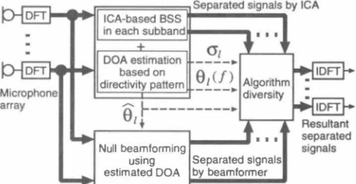
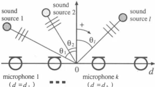
(2) where minx [ ，ν](max[x，叫) is defined as a function in order to obtain the smaller (larger) value among x and y. Based on these DOA inforrnations， we can detect and co汀ect the source perrnuta・ tion and the gain inconsistency.. sound. 2.2. Beamforming Section. microphone 1. (d. Figure. =. •••. d 1). In the beamforming section， we can construct an altemative un・ mixing matrix in parallel based on the null beamforming technique where the DOA information obtained in the ICA section is used. In the case that the look direction is 91 and the directional null is steered to 92， the elements of the unmixing matrix are given as. d. microphone k ( d dk ). =. 2: Confgi uration of microphone array and signals.. wrF)(ん) = exp[ -j21l}md1 sinÔl/c] x {exp[j2π!md1(sinÔ2 -sinÔ1)/C]. mixing matrix which is assumed to be complex-valued because we introduce the model to deal with the aπiving lags among each of the element of the microphone aηay and r∞m reverberations. We perforrn the signal separation by using the complex-valued unmixing matrix， W， so that the each element in the output Y W X becomes mutually independ巴nt in the case of K L. The optimal W can be obtained by using the following iterative 巴qua tion [4， 6):. =. =. Wi+1 =η(diag ((φ(y)yH))一(<þ(y)yH))(W r) -1 + W;. (2). where ( ) denotes the ave時ing operator， i is used to 巴xpress the value of the i th step in the iterations， and ηis the step size param eter. AIso， we defin巴 t山h巴 nonlinear ve伐削cαωtωoωr 仇釦伽Il肌I. ・. φ到(Y) = 1ν/パ{いl+ex功p(←一y(問R町))リ}+j .1ν/パ{いl+e位xp(←一y(仰Iり))リ}， (3). y(R). y(l). y，. where are the real and imaginary parts of re and spectively. Since the above-mentioned calculations are carried out at each frequency independently， problems about the source peロnutation and scaling indete口ninacy arise at every frequency bin. In order to resolve the problems， we have already provided the solution (4) to utilize the directivity pattem of the array system， Fì(f，θ)， which is is given by K. Fì(f，9) =乞 Wlk(f)叫[j21l}dk sin9/c]， k=1. (4). where C is the velocity of sound. Hereafter we assume the two channel case without loss of generality， i.e.， K = L = 2. In the directivity pattems， dir巴ctional nulls exist in only two particular directions. Accordingly， by obtaining statistics with respect to the directions of nulls at all frequency bins， we can estimate the DOAs of the sound sources. The DOA of the l th sound source， 91， can be estimated as. 81 =. N/2. 3 2: wm)， m=1. (5). where N is a total point of DFT， and 91(fm) represents the DOA of the 1 th sound source at the m th frequency bin. These are given by. 91(ん)=miベぽgqn|日(ん，9)1，釘ggLin|日(ん，9)1]，. (6). 92(ん)=mru伊g弓�n1日(ん，9)1刈g円�n1日(ん，8)1]，. (7). -exp[j2π!md2(SinÔ2-sinÔd/c]) - \ (8) wifF)(ん) = -exp[ -j2rr!md2 sinÔ1/C] x {exp[j2π!md1(sinÔ2 -sin Ô1)/C] 1 -exp[j2π!md2(SinÔ2 -sinÔd/C]}- ・(9) Also in the case that the look direction is 92 and the directional null is steered to 91， the elements of the unmixing matrix are given as. Wi�F)(fm) = - exp[ -j2rr!md1 sinÔ2/c] x {-exp[j2π!md1 (sinÔ1-sin Ô2)/C] 1 +exp[j2π!md2(sinÔ1-sinÔ2)/c]} - ， (10) wrF)(ん) = exp[ -j2rr!md2 sinÔ2/c] x { - exp[j2rr!md1 (sin Ô1-sinÔ2)/C] 1 +exp[j2π!md2(sinÔ1-sinÔ2)/C]} - . (11) 明1ese elements given by Eqs. (8)-(11) are norrnalized so that the each gain for look direction is set to be 1. 2.3. Integration of Subband ICA with Null Beamforming. In order to integrate the subband ICA with null beamforming， we newly introduce the following strategy for selecting the most suit able unmixing matrix in each frequency bin， i.e.， aIgorithm diver sity in the frequency domain. (1) If the directional null is steered to the proper estimated DOA of the undesired sound source， we use the unmixing matrix obtained by the subband ICA， Wl�CA)(f) . (2) If the directional null deviates from the estimated DOA， we use t山h児m削叩E引叩u山lßffilX幻in暗叩gma悶a瓜trix obt凶a幻i 耐 b句Y t山h巴 m凶 bear町mば帥nぱ的1ぜ由for口mロmin Iß pr，閃ef，先er陀enc巴 tωot山ha剖t of t山h巴 subband ICA. The above strategy yields the following algorithm:. )(f)， (1θl(f) - Ôd < h . 0"1) 2 1\ヌ C A\，':， Wlk(f) = f< W �' � -:主 h': ・ σV'I1)， (1 ) ::.'/'B �I， :'�J.� F ，I ' (1 ("(1) - 9d l WI�DrJ(f) where h is a magnification parameter of the threshold， and σ1 rep resents the deviation with respect to the estimated DOA of the 1 th sound source; it can be given as. ー N/2. σ1=川元乞 (θI(ん) - 81 )2. (1 3). nu nJUM.

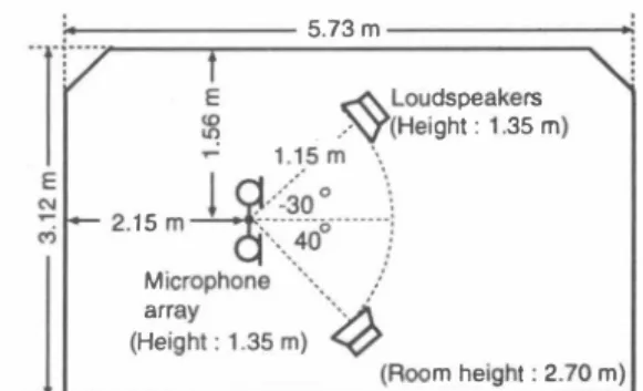
(3) お針. m. 25. c. 20. 5. 10. z. 5. o. 5 3 1. sec -----f子一 sec )(sec --→ー. _._ .-. -. -. 15. Q). -. �コ 2. =. 1. infinity. 2. Value of h. (Null beamfoming). (ICA-based BSS). Figure 4: Noise reduction rates for different values of threshold parameter h. Reverberation time is 0 msec. 9 7 6. �. 一ーーーーーーー』ー、、ー令. 、、、‘、、‘、、. 5. 3.2. Results 1: Effectiveness of Algorithm Diversity. 8 4. Learning duration. 3. { 国立 S 咽E c ouコ刀申庄申202. A two-element aπ'ay with the interelement spacing of 4 cm is as sumed.百e speech signals are assumed to arrive from two direc tions， -300卸d 400• Six sentences spoken by six male and six female speakers selected from the ASJ continuous speech co甲山 for research are used as the original speech. Using these sentences， we obtain 36 combinations with respect to speakers and source di rections. In these experiments， we used the following signals as the source signals: (1) the original speech not convolved with the impulse responses， and (2) the original speech convolved with the impulse responses recorded in two environments specified by dif ferent reverberation times (RTs)， 150 msec and 300 msec百le Im pulse responses are re氾orded in a variable reverberation time room as shown in Fig. 3. The analysis conditions of these experiments are summarized in Table 1.. m. Learning duration. 立30. æ. 3.1. Conditions for Experiments. )i m. 問問・明. 35 m. 0. 3. EXPERIMENTS AND RESULTS. 明 2 m 臼 t 同 k 問刷刷 b 。円 … 一妙。. m. Figure 3: Layout of reverberant r，∞m used in experiments.. 、、、、、、 ‘ 、有ム水 ‘ 』『 ‘ 『町半、、、、、、、、、、、、、、、、、、、、、. Using the algorithm with an adequate value of h， we can recover the unmixing matrix trapped on a local minimizer of the optimiza tion procedure in ICA. AIso， by changing th巴 parameter h， we can construct various types of訂ray signal processing for BSS， e.g.， a simple null beamforming with h =0，and a simpl巴 ICA-based BSS procedure with h =∞.. 2. o. =. 、. 、私. \. secー→子ー sec 持 sec一→一ー. 5 3 1. -ーー. 1. \\、. 、、 �fi�ty. 2. Value of h. (Null beamfoming). 、. (ICA-based BSS). Figure 5: Noise reduction rates for different values of threshold parameter h. Rev巴rberation time is 150 msec. 7 6 ー. 5. 占一. ‘. _.-ーーーー - . �. 一一. \ 、.、. ---ー--+、、、、. 4. 、、、.............. Learning duration = sec ー ..... ー sec -- →一ー + 、. 3. { 白Z S 国E EO冒Uコ33比申的一 oz. In order to illustrate the behavior of the proposed aπay for different values of h， the noise reduction rate (NRR)， defined as the output signal-to-nois巴 ratio (SNR) in dB minus input SNR in dB， is shown in Figs. 4-6. These valu巴s are taken as the average of all of the combinations with respect to speakers and source directions. The SNRs co汀espond to th巴 objective evaluation score in the case that the suppressed signal is r巴garded as noise. From Fig. 4 for the nonreverberant tests， it can be seen that the NRRs monotonically increase as the parameter h decreases， i.e.， the performance of the null beamformer is superior to that of ICA-based BSS. This indicates that the directions of the sound sources are estimated correctly by th巴 proposed method， and thus the null beamforming technique is more suitable for the separation of directional sound sources under nonreverberant condition In contrast， from Figs. 5 and 6 for the reverb巴rant tests， it is shown that (1) the NRR monotonically increases as the parameter h decreases in the case that the observed signals of 1 sec duration are used to leam the unmixing matrix， and (2) we can obtain the optimum performances by setting th巴 appropriate value of h， e.g.， h = 2， in the case that the leaming durations ar巴 3 and 5 sec. We can summarize from these results that the proposed combination algorithm of ICA and null beamforming is e仔ective for the signal separation， pa目icularly under the reverberant conditions.. 5 D 一O \ バ\ 日 /・ 3一. 8 kHz 32 msec 16 msec Hamming window 500 4 η= 1.0 X 10-. 江川 M M 出. Sampling Frequency Frame Length Frame Shift Window Number of Iterations Step Size Parameter. 5.73m. 一刷 14 F 3・ E t V、 v y h H. Table 1: Analysis Conditions of Signal Separation. 2. o. (Null beamfoming). 5 3 1. 持. ---f子一. sec. 1. 2. Value of h. .... ..... \、. infinity (ICA-based BSS). Figure 6: Noise reduction rates for different values of threshold parameter h. Reverberation time is 300 msec. τ14 ワ臼噌E4.

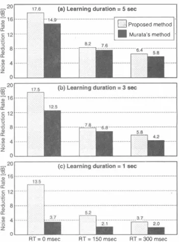
(4) 3.3. Results 2: Comparison with Conventional BSS Method. In order to perforrn a comparison with the conventional BSS method， we also perforrn the same BSS experiments using Murata's method [2]. Figure 7 (a) shows the results obtained using the proposed method and Murata's method where the observed signals of 5 sec duration are used to leam the unmixing matrix， Fig. 7 (b) shows those of 3 sec duration， and Fig. 7 (c) shows those of 1 sec duration. In these experiments， the parameter h in the proposed method is set to be 2. From Figs. 7 (a)ー(c)，in both nonreverberant and reverberant tests， it can be seen that the BSS perforrnances obtained by us・ ing the proposed method are the same as or superior to those of Murata's conventional method. In particular， from Fig. 7 (c)， it is evident that the NRRs of Murata's method degrade remarkably in the case that the leaming duration is 1 sec; however， there are no significant degradations in the case of the proposed method com pared with those of Murata's method. We can summarize the main reasons for the degradations in Murata's method by looking at the similarity (e.g.， cosine distance) among the sourc巴 signa1s of dif ferent lengths as follows (see Fig. 8). (1) The envelopes of the original source speech become more similar to each other as the duration of the speech shortens. (2) The separated signals' en velopes at the sam巴 frequency are similar to each other since the inaccurate unmixing matrix is estimated to hav巴many components of cross talk. Therefore， the recovery of the perrnutation tends to fail in Murata's method. In contrast， our method did not fail to recover the source pe口nutation because we did not use any infor mation of signal waveforrns but rather， used only the directivity pattems.. [4] S. Kurita，H. Saruwatari， S. K勾ita， K. Takeda，and F. Itakura， “Evaluation of blind signal separation method using directiv ity pattem under reverberant conditions，" Proc. JCASSP20ω， pp.3140-3143，2000. [5] Y. Karasawa，T. Sekiguchi， and T. Inoue，‘'The software an tenna: a new concept of kaleidoscopic antenna in multimedia radio and mobile computing era，" JEJCE Trans. Commun.， vo1.E80-B， nO.8，pp.1214-1217， 1997. [6] A. Cichocki and R. Unbehauen， “Robust neural networks with on-line learning for blind identification and blind sep aration of sources，" JEEE Trans. Circuits and Systems J， vol.43，no.l l ， pp.894-906，1996.. (a) Learning duration. =. 5鵠C. ロ Proposed method • Murata's method. 4. CONCLUSION. In this paper， a new blind source separation (BSS) method using subband independent component analysis (lCA) and beamform ing was described. In order to evaluate its e仔ectiveness， the signal separation experiments were perforrned under various reverberant conditions. From the results， it was shown that the noise reduction rate (NRR) of about 18 dB is obtained under the nonreverberant condition， and NRRs of 8 dB and 6 dB are obtained in the case that the reverberation times are 150 ms巴c and 300 msec. These perfor mances were superior to those of both simple ICA-based BSS and simple beamforming technique.. 5.2. RT. 5. ACKNOWLEDGEMENT. The authors are gratefu1 to Prof. Fumitada Itakura of Nagoya Uni versity for his suggestions and discussions on this work. This work was partly suppo口ed by a Grant-in-Aid for COE Research (No 11CE2005) and CREST (Core Research for Evolutional Science and Technology) in Japan. 6. REFERENCES. [1] A. Bell and T. Sejnowski，“An inforrnation-maximization ap proach to blind separation and blind deconvolution;' Neural Computation， vol.7， pp.1129-1159， 1995. [2] N. Murata and S. Ikeda，“An on-line algorithm for blind source s巴paration on speech signals， " Proc. of 1998 Jntema. 0 msec. RT. =. 150 msec. RT. =. 300 msec. =. 0.6 。. g. 0.5. 。. 0.4. �. 0.3. C cn 0 C. 0. 0.2. tional Symposium on Nonlinear Theory and Jts Application (NOLTA98J， pp.923-926， 1998.. [3] P. Smaragdis，“Blind separation of convolved mixtures in the frequency domain，" Neurocomputing， vol.22， pp.21-34， 1998.. =. Figur巴 7・ Comparison of noise reduction rates obtained by the proposed method (h 2) and Murata's method in the case that the leaming duration for ICA is (a) 5 sec， (b) 3 sec，and (c) 1 sec. X. 、、、、、. Separated -→子ー Original ---)(-. 、、、、、. 、、、、、. 、、、、、. 、、. ×ーーーーーーーーーー. 3. Speech Length [sec]. ーーーーーーーー×. 5. Figure 8: Cosine distances for different speech lengths. These values are the average of the all of the frequency bins.. 内〆山内ruM 可・ム.

(5)