近畿大学学術情報リポジトリ

全文

(1)Measuring the Catching Efficiency of Fishing Gear Yunosuke I ITAKA'. I Introduction. In order to manage fisheries intelligently it is necessary to have some knowledge of the capacity and efficiency of fishing gear. Fishing gears of different dimensions and designs not only differ in their sbsolu te ca tching capaci ties, bu t their relative efficiencies are a function of different species of catches, fishing season and ground operated, etc. The measurements and relative efficiency of fishing gears, here in compared are based on the statistical data u{- their own catches in replicated hauls on the same ground. In this paper, several statistical methods to measure the catching efficiency of fishing gear will be introduced. The writer wishes to express his hearty thanks to Capt. G. A. MOTTE, Department of Fisheries and Marine Technology, University of Rhode Island, U.S.A., for his kindness in reading the manuscript before printing.. It goes wi thou t saying that any statistical method is a technique to obtain, analyze and present" numerical data. For simple analysis the frequency distribution of data obtained should be "normal" and the variation should be about the same for all groups. It is therefore necessary to first examine the distribu tion of the catches by gear to determine if these requirements exist. If it is far from "normal", the data of the catches has to be adjusted properly in order that standard normal tests may be employed.. II Frequency Distribution of the Catches. Experience has shown that the catches in replicated hauls on the same ground by the same seine may be greatly different. This variability may be caused by a number of independent factors such as local movements of the fish shoals on the fishing grounds, diurnal variations in the availability of different species caught, slight changes in the conditions of fishing grounds and small changes in the behaviour of the seine in successive hauls. Thus, the frequency distribution of daily catches is far from "normal". YAMAMOTO (1956)1), based on his statistical data, pointed out that the frequency distribution of catches is approximately exponential or Poisson at the beginning and at the end of the season, and approaches "normal" in the middle of fishing period.. The following table (Table 1) is a score sheet to tally the daily catches, using the range of the catches as a guide, of 19 purse seiners operated in the Sea of Hyuga, Japan, at the 1955-season.. * Lab. of. Fishing Gear Technology, Dept. of Fisheries, Kinki Univ., Higashiosaka, Osaka 577. Japan. ". (Nj~J.J,tIIiJ. :. *~~Hi.tlt:ft.fiJf~~).

(2) 70 Table 1 Score Sheet of the Daily Catches of 19 Purse Seiners Operated in the Sea of Hyuga, Japan, 1955.. Daily Catches (Baskets*) (Class In tervals). Tally. Frequency. 0-50. 92. 51 - 100. 130. 101-150. 91. 151- 200. 65. 201-'-250. 45. 251 - 300. 26 21 18 10 6 14 6 6 8 5. 301- 350 351- 400 401 - 450 451 - 500 501 - 550 551 - 600 601 - 650 651 - 700 701 -750 751- 800 801 - 850 851 - 900 901 - 950 951-1000 1000 - over Total. I I. o I 5. o 551. * One "Basket" is about 30 kg in weight.. Fig. 1 is the graphic presentation of Table 1. A glance at Table 1 and Fig. 1 is enough to show that the frequency distribution of daily catches is far from "normal" and is a right skewed one which distorts the curve towards the right. This type of distribution may be considered very approximately exponential. If this is exponential, the appropriate adjustment of the data (daily catches) is made by some form of logarithmic or square root transformation. Some other transformations than these two are considered, but these are well-known and are convenient for calculation .. .\ ...

(3) 71. Y.litaka: Measuring the Catching Efficiency of Fishing Gear Frequency 130. 120 110 100 90 80. 70 60 50. 40 30 20 10. 00 Catches per Day (Baskets) Fig. 1 Distribution (Histogram) of Daily Catches of 19 Purse Seiners Operated in' the Sea of Hyuga, Japan, 1955. - Data in Table 1 Frequency. Frequency. 110. 110. -. 100. -. 90. ~. 100. r--. c0-. 90. 80. 80. 70. 70. l-r--. ~. I--. 60. 60. r--. 50. 50. 40. 40. ,--. -. co-. 30. 30. r--. 20 10. o. r-rniT. 20. -,--. 10. 0.4000.800 1.200 1.6002.0002.4002.800 3.200,. oo. Log-Values of Catches Fig. 2 Distribu tion where the Daily C·a tches are converted to Logarithmic Values. - Data from Table 1 -. .'.. 5.0 10.0. ~. 15.0 20.0 25.0. 30.0 35.0. Root-Values of Catches Fig. 3 Distribution where the Daily 'Catches are converted to Square Root Values. - Data from Table 1 -. '-. ..

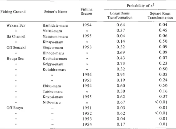
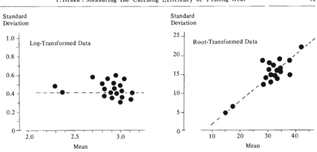
(4) 1f, 7~' (1974). 72. A logarithmic transformation was used by PARRISH (1951)2) to adjust the trawl catch data in his study. KIMURA (1932)3) in his analysis of the yellowtail fishery used the square root transformation to adjust the observed distributions. Fig. 2 is the frequency distribution in which the daily catch data are converted to logarithmic values. Fig. 3 is the frequency distribution of the square root transformations. It can not be said surely from Figs. 2 and 3, which transformation, the logarithmic or the square root, fits the "normal" better. In order to determine which transformed data is most normally distributed, a Chi Square Test CX2-Test) was made by IITAKA (1956)4), based on the daily catches of 19 purse seiners operated in different waters off Japan. The results are tabulated in Table 2. It can be seen from the above table that in almost all cases, 14 ou t of 19 cases, the logarithmic transformation fits much better than the square root transformation. In addition to the above, the relationship between the standard deviation and the mean of catches, of the logarithmic and the square root transformations, were examined by the writer and shown in Fig. 4. Fig. 4 indicates that the standard deviation obtained by the logarithmic transformation seems to be nearly constant regardless of the mean of catches, whereas the standard deviation in the case of the square root transformation increases as the mean of catches increases. It is, therefore, concluded that the frequency distribution of daily catches by a seine is approximately exponential and that the logarithmic transformation of the catch data would give the better results when assessing statistically the relative catching efficiencies of gears.. Table 2. Results of the x 2 -Test to determine the Fitness of Transformed Data OITAKA, 1956)4). Probability of x 2 Fishing Ground. Seiner's Name. Fishing Se<\son. Wakasa Bay. Hashida te-maru. 1954. Iki Channel Off Senzaki Hyuga Sea. Meisei-maru Masu tomi-maru Kinsyo-maru Singyo-maru. 1955 1953. Hinode-maru Kyohuku-maru Keigyo-maru Kotohira-maru. 1954 1955 1954. Ebisu-maru Taisyu-maru Koyosi-maru Nitto-maru. 1955 1951 1952 1953 1954. Off Bosyu. :(. ;.. I. '. Logarithmic Transformation. 0.64 0.37 0.04 0.14 0.32 0.69 0.43 0.73 0.32 0.95 0.19 0.60 0.30 0.62 0.67 0.03 0.62 0.04 0.17. Square Root Transforma tion. 0.04 0.45 0.06 0.50 0.09 0.09 0.07 0.23 0.80 0.05 0.24 0.50 0.16 0.37 < 0.01 0.01 <0.01 0.01 0.01.

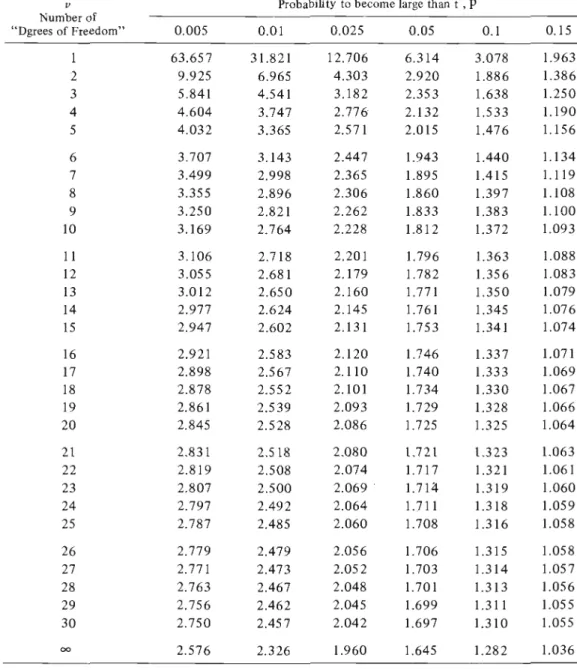
(5) 73. Y.litaka : Measuring the Catching Efficiency of Fishing Gear Standard Deviation. Standard Deviation 1.0. 25 Root-Transformed Data. Log-Transformed Data 20_. 0.8 0.6. -.-. •. -- -. 0.4 -. -. 0.2 -. •••• • •• - - ~.\.-.-•••• •. 15 10. -. 5 /. /. o. o. 1. 2.0. 2.5. 3.0. 1. I. I. i. 10. 20. 30. 40. Mean. Mean. Fig. 4 Relation between the Standard Deviation and the Mean of Catch~s, in the Cases of Logarithmic and Square Root Transformations. - Data from Table 2 -. III Application of the "Student t-Test". Very frequently it is desirable to test the difference in catches between two gears to determine whether there is any significant difference, or whether the difference, if any, is merely due to chance. In these cases, the "Student t-Test" may be used. If two samples of any data are drawn from a same population undoubtedly, the true difference between two samples is in reality zero. If any differences happen between the samples, it is only due to accidence or chance. Generally, the value of: t. = (x -m)j"i1T s. where. x = the mean of sample. x. m = the mean of entire population n = the number of sample x s = the standard deviation of sample x. gives the distribution of "Student t" where the number of "degree of freedom" is v = (n - 1). On the other hand, the values of t are tabulated in Table 3 by number of "degrees of freedom" and the probability due to chance. It is, therefore, easy to measure the significance between two samples, from the comparison with the values obtained above and in Table 3. For instance, let x be the difference between two groups. Set up a hypothesis that two groups are drawn from the same population, that is,. m=O. Thus, we can get. x''i1=T t =_--,-"'_11-_ J_ s.

(6) i1I. 74. ~. * ¥:. J:l< :j.: :~:;. *c. ~. W, 7 f;. (1974). Table 3. Distribution of the Student t Values by the Probability and the Number of "Degrees of Freedom" (HOEL, 194 7)S).. Probabili ty to become large than t , P. v. Number of "Dgrees of Freedom". 0.005. 0.01. 0.025. 0.05. 0.1. 0.15. 1 2 3 4 5. 63.657 9.925 5.841 4.604 4.032. 31.821 6.965 4.541 3.747 3.365. 12.706 4.303 3.182 2.776 2.571. 6.314 2.920 2.353 2.132 2.015. 3.078 1.886 1.638 1.533 1.476. 1.963 1.386 1.250 1.190 1.156. 6 7 8 9 10. 3.707 3.499 3.355 3.250 3.169. 3.143 2.998 2.896 2.821 2.764. 2.447 2.365 2.306 2.262 2.228. 1.943 1.895 1.860 1.833 1.812. 1.440 1.415 1.397 1.383 1.372. 1.134 1.119 1.108 1.100 1.093. 11 12 13 14 15. 3.106 3.055 3.012 2.977 2.947. 2.718 2.681 2.650 2.624 2.602. 2.201 2.179 2.160 2.145 2.131. 1.796 1.782 1.771 1.761 1.753. 1.363 1.356 1.350 1.345 1.341. 1.088 1.083 1.079 1.076 1.074. 16 17 18 19 20. 2.921 2.898 2.878 2.861 2.845. 2.583 2.567 2.552 2.539 2.528. 2.120 2.110 2.101 2.093 2.086. 1.746 1.740 1.734 1.729 1.725. 1.337 1.333 1.330 1.328 1.325. 1.071 1.069 1.067 1.066 1.064. 21 22 23 24 25. 2.831 2.819 2.807 2.797 2.787. 2.518 2.508 2.500 2.492 2.485. 2.080 2.074 2.069 . 2.064 2.060. 1.721 1.717 1.711 1.708. 1.323 1.321 1.319 1.318 1.316. 1.063 1.061 1.060 1.059 1.058. 26 27 28 29 30. 2.779 2.771 2.763 2.756 2.750. 2.479 2.473 2.467 2.462 2.457. 2.056 2.052 2.048 2.045 2.042. 1.706 1.703 1.70 I 1.699 1.697. 1.315 1.314 1.313 1.311 1.310. 1.058 1.057 1.056 1.055 1.055. 00. 2.576. 2.326. 1.960. 1.645. 1.282. 1.036. 1.71~. Note: when the absolute value is used, the probability must be doubled.. (' ,. ,. ,. ..

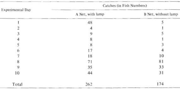
(7) 75. Y.litaka: Measuring the Catching Efficiency of Fishing Gear. where v = (n - 1). From Table 3, we obtain the value corresponding to the above at any standard probability level. If the calculated value of t is larger than the one obtained from Table 3, the hypothesis may be said to be false at the confidence level used. The populations of the two groups are then different from each other, and the difference between both is significant and not due to chance at the selected probability.. Example 1 Consider the data of the daily catches by two fixed nets set in the same fishing ground, as shown in Table 4. The two nets are the same in their dimensions and designs, while only one of them used a fish-lamp. Which net is better in catching capacity? Table 4. Daily Catches of Two Fixed Nets (SASAKI and WATANABE, 1948)6).. Catches (in Fish Numbers) Experimental Day A Net, with lamp. 1 2 3 4. 5. 48 4 9 8 8 17 18 71. B Net, without lamp. 5 1 5 1. 3 4. 6 7 8 9 10. 44. 33 31. Total. 262. 174. 35. 10 81. Assuming the frequency distribution of daily catches by two nets is approximately logarithmic normal (as discussed in the previous chapter), the data are first converted to common logarithmic values (Use Table 11). In this case, the logaritluns of the original data (fish numbers caught) plus one are used, e.g. if the original data is N, log (N + I) is used, thus avoiding ambiguity when data is zero. The procedure for calculating t is shown in Table 4a..

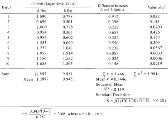
(8) 76 Table 4a. The Student t-Test. - Data from Table 4 Catches (Logarithmic Value). Day, i 1 2 3 4 5 6 7 8 9 10. Sum. A Net. B Net. Difference between A and B Nets, x. Value of x 2. 1.690 0.699 1.000 0.954 0.954 1.255 1.279 1.857 1.556 1.653. 0.778 0.301 0.778 0.301 0.602 0.699 1.041 1.914 1.532 1.505. 0.912 0.398 0.222 0.653 0.352 0.556 0.238 -0.057 0.024 0.148. 0.832 0.158 0.0493 0.426 0.124 0.309 0.0567 0.0033 0.0006 0.0219. 9.451 0.9451. L'x = 3.446 iMean x = 0.3446. 12.897 Mean 1.2897. L x 2 = 1.981 i. Square of Mean. :X 2 = 0.119 Standard Deviation S = JO/lO) 1.981-0.119 t. 0.345~ 0.281. = 0.281. =-----,--- = 3.68 where v = 10- 1 = 9 '. On the other hand, from Table 3 we can get the value corresponding to the above as t = 1.833. where v = 9 and the probability p = 0.05. As 3.68 is larger than 1.833, it may be said that the difference in catches between two nets is significant at the probability of 0.05. In order to check the confidence limit of the mean x, at the 95% confidence limit, the following inequality is considered:. (x - m)jn=T s. I. < t(o.OS). that is,. _ s s x - t(o.OS).;n=T <m <x + t(o.OS) jn -1. where t(o.OS) means the absolu te value of t at the probability of 0.05..

(9) 77. Y. Iitaka.: Measuring the Catching Efficiency of Fishing Gear. In Table 3 we obtain t(0.05). = 2.262. where v = 9 (Note: in Table 3 when the absolute value is used, the value of probability p must be doubled). Thus, we have 0.345 - 2.262. 0.281. 0.281. jiO""="l < m < 0.345 + 2.262 "jl;=;;O=_=:'J=-. that is, 0.133 < m < 0.557 Clearly from the above result, it can not be said positively with 95% confidence that the net with a lamp may catch over (. 0~9~:1. x 100). = 14%. more than the net without a lamp.. To test the significance of the difference between two means of samples, the same treatment would be used. In this case, the hypothesis that two samples are drawn from the same population can be set up. Let X, si and n x be the mean, the variation and the number of one of the samples x, respectively. Symbols )I, sJ" ny are those of the other sample y. m x and my are the means of the two populations. The value of t. = (x -)I) -2. (m x -my) nxSx + nysy2. ---'-----F~~~"..-;;...:...-. J. nxny (n x + ny -2) n x +n y. gives the distribution of "Student t" where the number of "degree of freedom" v is (n x +ny - 2). Since the hypothesis is we get. x-y. t. = j nxsx2 + nySy2. nxny (n x + ny - 2) n x +ny. Thus the confidence interval for (m x -my), will be as follows:. (x -f) -. t(0.05). Obviously if the above hypothesis is false then the alternative view is taken and m x. ! .J. f- my..

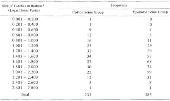
(10) 78. :;~. 7. f; ( I 9 7 4 ). Example 2 The statistical data in daily catches of 14 purse seiners operating in the Sea of Hyuga, Japan, 1965, is shown in Table 5. All seines are almost the same in their dimensions and designs. However, 8 of them were made of cotton twine, while the rest were made of Kyokurin (a mixture of Saran, polyvinyliden chloride, and Nylon, polyamide, filaments) twine. Let us compare which group of seines is significantly better in catching efficiency. Table 5. Distribution of the Daily Catches by Size, in Two Groups of Seiners, 1965.. Size of Ca tches in Baskets * (Logarithmic Value). 0.001 0.201 0.401 0.601 0.801 1.001 1.201 1.401 1.601 1.801 2.001 2.201 2.401 2.601. -. Frequency Cotton Seine Group. 0.200 0.400 0.600 0.800 1.000 1.200 1.400 1.600 1.800 2.000 2.200 2.400 2.600 2.800. * one "Basket". 1. o o. 9 12 16. 5 11. 23 32. 29 39. 1. 34 37 30. 22 12 3. Total. Kyokurin Seine Group. 1. 57 68 74 59 31. 8. 1. 1. 233. 383. is about 30kg in weight.. In Table 5 the data are converted to common logarithmic values, assuming the frequency distribution of original data (in baskets) is exponential. Since sizes are used as ranges of the data, the midpoint of the class interval is taken as the value of x or y. In this case the values of x and S2 are calculated as follows:. x= lLxf n. where f is a frequency number. The procedure of calculation for t is shown in Table Sa..

(11) 79. Y. litaka : Measuring the Catching Efficiency of Fishing Gear Table 5a The Student t-Test. - Data from Table 5 . Frequency. Catches-Midpoint of. Size (Log-Value) x or y. 0.100 0.300 0.500 0.700 0.900 1.100 1.300 1.500 1.700 1.900 2.100 2.300 2.500 2.700. Callan Group fx. Kyokurin Group fy. I I. 0 0 1 5. 9 12 16 23 32 34 37 30 22 12 3. II. 29 39 57 68 74 59 31 8 1. I n x = 233. Sum. xfx. 0.1 0.3 4.5 8.4 14.4 25.3 41.6 51.0 62.9 57.0 46.2 27.6 7.5 2.7. n y = 383 'J:,xlx. Yfy. x 2 or y2. 0 0 0.5 3.5 9.9 31.9 50.7 85.5 115.6 140.6 123.9 71.3 20.0 2.7. 0.01 0.09 0.25 0.49 0.81. x 2f x. 0.01 0.09 2.25 5.88 12.96 27.83 54.08 76.50 106.93 108.30 97.02 63.48 18.75 7.29. 1.2 I. 1.69 2.25 2.89 3.61 4.41 5.29 6.25 7.29. 'J:,Yly. = 349.5 = 656.1. 2 'J:,x lx. y2fy. 0 0 0.25 2.45 8.91 35.09 65.91 128.25 196.52 267.14 260.19 163.99 50.00 7.29 'J:,y. 2. f. = 581.37 = 1185:99. Y '" _1_ 'J:,Yly = (1/383) x 656.1 x = -1-'J:,~/x = (1/233) x 349.5 = 1.500 n y. nx 2 2 2 y2 = 1.713 = 2.934. x = 1.500 = 2.250 2 2 2 sx = _1_ 'J:,x Ix - x = (1/233) x 581.37 - 2.250 = 0.245 n. = 1.713. x. sy 2 = _1 'J:,y2ly _ y2 = (1/383) x 1185.99 - 2.934 = 0.163 ny. = t. 1.713-1.500 J233xO.245+383xO.163 x. 233x383x(233+383-2) =581 where 233+383 .,. =233+383-2 II. On the other hand, from the "Student t" distribution (Table 3), we get t = 2.326. where II = 00 and p = 0.01. lt can be said that the hypothesis is false because the calculated t is larger and the difference between two groups of seines, cotton and Kyokurin, is significant. The 95% confidence limit of the difference between two means is. (1.713 _ 1.500)- 1.960 x )233 x 0.245 + 383 x 0.163. 233 x 383 (233 + 383 - 2). 233 + 383. < mx that is,. my. <. < (1.7 I 3 -. <. J233 x 0.245 + 383 x 0.163 1.5 00) + 1. 960 x ~~~=c==c=:=============- 233 x 383 (233 + 383 - 2) 233 + 383. 0.141 m x - my 0.285 From the above result it may be said with 95% confidence, that the catch of a purse seine may be expected to increase about 10% by changing from cotton to Kyokurin in material.. '. J.

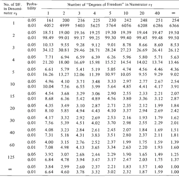
(12) J!.Iw!f*·tl~:'¥:fil)*c~. 80. ;r;. 7. ~. (1974). IV Application of the "Analysis of Variance". When the variation of data is expected to be caused by several independent factors, the statistical method of "Analysis of Variance" should be used in order to check its significance. It is carried out to compare the contribution to the variation due to each factor with the overall random term called "error", using the F-Test. The unbiased variances of some selected terms, including the error variance, are calculated first. Then the ratio of the unbiased variances to the error term may be obtained. These ratios are called the "Testing Factors" and are compared with the corresponding F value in Table 6, where the values of F are tabulated by the numbers of "Degree of Freedom" and by some standard probability leveL If any calculated "Test Factor", F is larger than the corresponding value in Table 6, the variance is significant. The unbiased variance is represented by: Sum of Squares by Source Number of "Degree of Freedom" Table 6. Distribution of the F Values by the Probability and the Numbers of "Degrees of Freedom';. (HOEL, 1947)5). No.ofDF. in Denominator V2. Proba bility. Number of "Degrees of Freedom" in Numerator. Vf. 1. 2. 3. 4. 5. 10. 20. 40. 0.05 0.01. 161 4052. 200 4999. 216 5403. 225 5625. 230 5764. 242 6056. 248 6208. 251 6286. 254 6366. 2. 0.05 0.01. 18.51 98.49. 19.00 99.01. 19.16 99.17. 19.25 99.25. 19.30 99.30. 19.39 99.40. 19.44 99.45. 19.47 99.48. 19.50 99.50. 3. 0.05 0.01. 10.13 34.12. 9.55 30.81. 9.28 29.46. 9.12 28.71. 9.01 28.24. 8.78 27.23. 8.66 26.69. 8.60 26.41. 8.53 26.12. 4. 0.05 0.01. 7.71 21.20. 6.94 18.00. 6.59 16.69. 6.39 15.98. 6.26 15.52. 5.96 14.54. 5.80 14.02. 5.71 13.74. 5.63 13.46. 5. 0.05 0.01. 6.61 16.26. 5.79 13.27. 5.41 12.06. 5.19 11.39. 5.05 10.97. 4.74 10.05. 4.56 9.55. 4.46 9.29. 4.36 9.02. 10. 0.05 0.01. 4.96 10.04. 4.10 7.56. 3.71 6.55. 3.48 5.99. 3.33 5.64. 2.97 4.85. 2.77 4.41. 2.67 4.17. 2.54 3.91. 15. 0.05 0.01. 4.54 8.68. 3.68 6.36. 3.29 5.42. 3.06 4.89. 2.90 4.56. 2.55 3.80. 2.33 3.36. 2.21 3.12. 2.07 2.87. 20. 0.05 0.01. 4.35 8.10. 3.49 5.85. 3.10 4.94. 2.87 4.43. 2.71 4.10. 2.35 3.37. 2.12 2.94. 1.99 2.69. 1.84 2.42. 30. 0.05 0.01. 4.17 7.56. 3.32 5.39. 2.92 4.51. 2.69 4.02. 2.53 3.70. 2.16 2.98. 1.93 2.55. 1.79 2.29. 1.62 2.01. 40. 0.05 0.01. 4.08 7.31. 3.23 5.18. 2.84 4.31. 2.61 3.83. 2.45 3.51. 2.07 2.80. 1.84 2.37. 1.69 2.11. 1.51 1.81. 60. 0.05 0.01. 4.00 7.08. 3.15 4.98. 2.76 4.13. 2.52 3.65. 2.37 3.34. 1.99 2.63. 1.75 2.20. 1.59 1.93. 1.39 1.60. 125. 0.05 0.01. 3.92 6.84. 3.07 4.78. 2.68 3.94. 2.44 3.47. 2.29 3.17. 1.90 2.47. 1.65 2.03. 1.49 1. 75. 1.25 1.37. 00. 0.05 0.01. 3.84 6.64. 2.99 4.60. 2.60 3.78. 2.37 3.32. 2.21 3.02. 1.83 2.32. 1.57 1.87. 1.40 1.59. 1.00 1.00. ,.. \ •. I. 00.

(13) 81. Y. Iitaka : Measuring the Catching Efficiency of Fishing Gear. Suppose where the variability of catch data Xij is considered to be due to two systematic causes; ground and gear. The symbol i shows as a fishing ground, while j is a fishing gear, as shown in below: Gears. 2 I 2. Grounds. a. j. b. XII X21. X12. Xlj. X22. X~j. xlb x2b. XI' X2'. xii. Xi2. Xii. Xib. Xi-. Xal. Xa2. Xaj. Xab. Xa'. X'I. X·2. x'j. X·b. X. In this case the total sum of squares of data is. ~~(Xij_X)2 = ~~xi7I J I J. I. ab. (~~Xij)2 I J. The sums of squares by ground and gear are, respectively 1. b~(Xi' _X)2 = b ~(~Xij)2 I. I. J. -. ---L (~'f;,xij)2 ab. J. I. and. a~(x. '_X)2 =-.l ~(~x·y - ~ (~~x·y j J a j i IJ ab i j IJ On the other hand, since the sum of squares by "error" is equal to the value of total sum minus the sums of the ground and the gear, ~~(Xij _X)2 -b~(Xi' _X)2 -a~(x. j _X)2 I J I I. The numbers of "Degree of Freedom" are (ab - 1) for total, (a - 1) for ground and (b - 1) for gear. Therefore, for "error" we get (ab - 1) - (a - 1) - (b - 1) Thus, we can get the values of the "Test Factor" for the two factors, ground and gear, as shown below: for ground,. F ground. a-I = ---------=-------'=----=---:-------:: ~~(Xij _X)2 -b~(Xi' _X)2 -a~(x.j _X)2 I. J. I. J. (ab - 1) - (a -1) - (b -1). where the numbers of "Degree of Freedom" are in numerator VI =(ab - 1) - (a - 1) - (b - 1), and for gear,. =a-I. and in denominator. V2. a~(x.j-x)2 J. (ab - 1) - (a - 1) - (b - 1) where the numbers of "Degree of Freedom" are in numerator VI V2 = (ab -1) - (a -1) - (b -1).. I ." " J. =b -. 1 and in denominator.

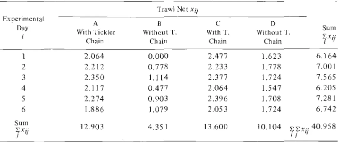
(14) ,~"i. 82. 7 ,;. (1 974 ). Example 3 Table 7 shows the catches per haul for six successive days by 4 trawl nets, examined in Europe (PARRISH, 1951 F). The values in Table 7 are all converted into logarithmic values, assuming the frequency distribution of the catches is exponential. Compare the difference in the catching capacities of the 4 nets by means of the "Analysis of Variance". Two nets, A and B, are the same, but A only used a tickler chain. Similarly, C and D nets are the same, but C only used a tickler chain.. Table 7. Catches per Haul in the Logarithmic Values by 4 Trawlers (Parrish, 1951)2). Trawl Net xii Experimental Day. A. B. With Tickler Chain. Without T. Chain. C With T. Chain. D Without T. Chain. 2.064 2.212 2.350 2.117 2.274 1.886. 0.000 0.778 1.114 0.477 0.903 1.079. 2.477 2.233 2.377 2.064 2.396 2.053. 1.623 1.778 1.724 1.547 1.708 1.724. 6.164 7.001 7.565 6.205 7.281 6.742. 12.903. 4.351. 13.600. 10.104. LLx··40.958 i i II. 1 2 3 4 5 6 Sum LX" i II. Sum LX" i II. The practical procedure of calculations of Fday and F net is shown in Table 7a. The values in Table 7a are square numbers of the values in Table 7. Table 7a F-Test..- Data from Table 7 2. Trawl Net xii,. Experimental Day i, a = 6. 1 2. D. 0.000 0.605 1.241 0.228 0.815 1.164. 6.136 4.986 5.650 4.260 5.741 4.215. 2.634 3.161 2.972 2.393 2.917 2.972. 166.487. 18.931. 184.960. 102.091. 27.886. 4.053. 30.988. 17.049. 3. ~xi. i II. C. 4.260 4.893 5.523 4.482 5.171 3.557. 4 5 6 (LX·")2. B. A. b = 4. = 1677.558. ~(ix-)2. ~(Lx·")2 =. = 281.208. i. '1. (L LX··)2 i i II. L LX~' = 79.976 i. .f.. 37.995 49.014 57.229 38.502 53.013 45.455. i. II. i II. 472.469. i. i. II.

(15) Y.litaka: Measuring the Catching Efficiency of Fishing Gear. The sums of squares by: bf(Xi- _X)2. day;. =+281.208. -6~ 4. 1677.558. = 70.302 - 69.898 = 0.404 I 1 =6472.469-6"><41677.558. 2. net;. af(x'i-x). error;. 4~(Xii-x)2 -b'i;(Xi.-X)2 -a4-(x.j-x)2. = 78.745 - 69.898 = 8.847 f. I. f. I. =4-4-xij--bl (4-4 Xzj)2_ 0 .404-8847. a. f. I. = 79.976 - 6. I. ~. f. 4 1677.558 - 0.404 - 8.847 = 0.827. Thus, we have "Test Factors":. F. day;. VI. da Y. net;. F net. V2. VI. V2. 0.404 --'6'--------'1=-_ =IS0.827 .,---,-----,-----,-----.,---,-----,-----,--------(6 x 4 - I) - (6 - I) - (4 - I) 8.847 = 3 4-1 = IS -----0-.8-2-'7-- - - - - = (6x4-1)-(6-l)-(4-1). =. 5. 0.081 = I 47 0.055 .. 2.949 0.055 = 53.6. On the other hand, from Table 6: F. VI = 5 V2 = IS. = 2.90 at the probability of 0.05. F. vI V2. =. = 3.29 at the probability of 0.05. 3. = IS. It can be said from the above results that the variance in catches due to the difference between nets is very significant. This may be caused by fishing with a tickler chain or without. A confidence interval on the means for day or net may be calculated as described in the previous or following chapters.. V Application of the "Least Squares Method" The "Least Squares Method" may be applied to compare the catching capacities of several fishing boats. Let the symbol Xzj be the catches by the j-th boat at the i-th day, and xi. be the mean catches by boats operated at the i-th day. If (Xi is the index number representing the relative catching efficiency of the j-th boat, the following relation may be satisfied: xij = (XixiTherefore, by means of the "Least Square Method", the value of (Xi may be determined so that the sum of the squares of the deviations (the differences between xij and (XiXi-) will be a minimum. That is,. Thus, we have (Xi =. 4 XljXi-. ~x? I. 83.

(16) 84 Example 6 Given the statistical data of catches by six seiners as shown in Table 8, estimate the relative catching indexes of those seiners. Table 8. Daily Catches (Cases) in the Logarithmic Values by 6 Seiners (TAUT!, 1956) 7).. Seiner j,. Day I. 2 3 4 5 6. Xij. Sum I:x". A. B. C. D. E. F. 1.204 1.079 0.954 1.556 1.301 1.681. 1.397 0.477 1.279 1.643 0.954 0.602. 0.954 0.000 0.845 1.579 0.778 1.568. 0.954 0.700 1.041 1.556 1.041 0.301. 0.778 1.000 1.477 1.556 1.114 0.845. 1.000 0.602 1.041 1.716 1.380 0.301. j. II. 6.287 3.858 6.637 9.606 6.568 5.298. Note: One case is about 4 kg in weight. The procedure for calculation is as shown in Table 8a. The values in Table 8a are as calculated.. Xi/Xi.. Table 8a Estimation of the Relative Catching Index. - Data from Table 8 -. Seiner j,. Day A. I 2 3 4 5 6 '2;Xij X i' I. '2;xij X i· CXj=. 2. I. '2; xi·. XijXi·. B. C. D. E. 1.262 0.694 1.055 2.491 1.425 1.484. 1.464 0.307 1.415 2.630 1.045 0.532. 1.000 0.000 0.935 2.528 0.852 1.385. 1.000 0.450 1.151 2.491 1.140 0.266. 0.815 0.643 1.634 2.491 1.220 0.746. 1.048 0.387 1.151 2.747 1.511 0.266. 8.411. 7.393. 6.700. 6.498. 7.549. 7.110. F. -2. xi-. xi·. 1.048 0.643 1.106 1.601 1.095 0.883 '2;x? =. 1.098 0.413 1.223 2.563 1.199 0.780 7.276. I. 1.16. 1.02. 0.92. 0.89. 1.04. 0.98. I. It is considered that the relative catching indexes of the 6 seiners, A, B, C, D, E and Fare 1.16, 1.02,0.92,0.89, 1.04 and 0.98, respectively.. Example 7 Table 9 shows the daily catches by seven seines. The total number ofseines operated on the same day and their total catches are also tabulated in Table 9. Let us estimate the relative catching indexes of those seines.. The procedure for calculation is as described in Table 9a. In this case, the days in which any of the seven seines did not operate, have been removed. The values in Table 9a are the logarithmic values of the catch data shown in Table 9, and the parenthesized values are calculated from x ij Xi· ..

(17) 85. Y.litaka: Measuring the Catching Efficiency of Fishing Gear Table 9. Daily Catches (Cases) by 7 Seiners and Total Catches and Number of Seiners Operating on the Same Day (TAUTI, 1956)7).. By All Seiners Operated Date (1951 ). I, 4 5, 4 9, 4 14, 4 21, 4 27, 4 3, 5 10, 5 15, 5 21, 5 4, 6 13, 6 23, 6 30, 6 7, 7 17, 7 20, 7 30, 7 7, 8 15, 8 24, 8 27, 8 3, 9 10, 9 17, 9 26, 9 2, 10 11,10 19,10 30,10 6, II 13, II 20, II 25, II 6, 12 10, 12 17, 12 25, 12. By 7 Seiners, each. Total Catches. Number of Seiners. Mean Catches. 184 170 648 310 3156 1264 7008 19920 17276 24648 6324 6196 6730 1088 4330 3416 3250 3860 1148 1698 1178 4070 2676 280 182 270 84 220 1822 1114 6436 2492 1124 10264 525 736 5748 2632. 28 17 44 65 71 72 90 121 110 126 122 132 71 14 81 74 60 75 46 46 48 35 72 15 14 62 70 30 70 43 83 80 80 91 57 90 87 95. 6.57 10.00 14.73 4.77 44.45 17.56 77.87 164.63 157.05 195.62 51.84 46.94 94.79 77.71 53.46 46.16 54.17 51.47 24.96 36.91 24.54 116.29 37.17 18.67 13.00 4.35 1.20 7.33 26.03 25.91 77.54 31.15 14.05 112.79 9.21 8.18 66.07 27.71. Note: One case is about 4 kg in weight.. .r... /. A. B. C. D. E. F. 40. 960. G. 16 16 20 32. 48. 92. 136 280. 152. 304. 104. 10. 96. 40 168 10 64 8. 20 4 8 6. 16 12. 76 88 32. 32 273 4 4 64. 4. 56.

(18) i!I ~. 86. *. 'j:. C ? :t~. *C. ~. :;.;. 7~;'. (1 9 7 4 ). Table 9a Estimation for the Relative Catching Index. - Data from Table 9 -. Date (1951). Seiner,j, Xij. (XijXi.) -2. Xi·. xi·. 4. 0.818. 0.669. 5, 4. 1.000. 1.000. 9, 4. 1.167. 1.362. 14, 4. 0.679. 0.461. 2J, 4. J.648. 2.7 J6. 3, 5. 1.892. 3.580. 10, 5. 2.218. 4.920. 15, 5. 2.196. 4.822. 13, 6. 1.671. 2.792. 20, 7. 1.734. 3.007. 30, 7. 1.712. 2.931. 7, 8. 1.398. 1.954. 15, 8. 1.567. 2.455. 24, 8. 1.389. 1.929. 3, 9. 1.571. 2.468. 17, 9. 1.114. 1.241. 26,. 9. 0.639. 0.408. II, 10. 0.865. 0.748. 19,10. 1.415. 2.002. 6, 11. 1.889. 3.568. 13, II. 1.494. 2.232. 25, II. 2.053. 4.215. 6,12. 0.964. 0.929. 10,12. 0.910. 0.828. 25, 12. 1.443. 2.082. i. I,. A. B. C. D. E. F. 1.602 (2.640). 2.982 (4.9J4). G. 1.204 (0.985) 1.204 ( 1.204) 1.301 (1.518) 1.505 ( 1.022). 1.964 (3.716). 1.681 (3.180). 2.134 (4.038) 2.447 (5.427) 2.483 (5.453) 2.017 (3.370). 1.000 (1.712). 2.182 (4.840). 1.982 (3.312). 1.602 (2.778) 2.225 (3.809) 1.000 ( 1.398) 1.806 (2.830) 0.903 ( 1.254). 1.301 ( 1.807) 0.602 (0.946) 0.903 ( 1.006) 0.778 (0.497). 1.204 ( 1.041) 1.079 (1.5 27). 1.881 (2.662) 1.945 (3.674) 1.505 (2.248). 1.505 (2.248) 2.436 (5.001) 0.602 (0.580) 0.602 (0.548) 1.806 (2.606). .! . • 1. 0.602 (0.869). 1.748 (2.522).

(19) 87. Y.Iitaka: Measuring the Catching Efficiency of Fishing Gear. 0.985 + 3.716 + 1.712 + 2.662 + 2.248 0.669 + 3.580 + 2.931 + 2.002 + 2.232 11.323 11.414 0.99 8.919 = I 03 1.000 + 3.007 + 2.931 + 0.929 + 0.828 8.695 . <Xc = 1.518+3.180+2.830+3.674+2.606 = 13.808 = 106 1.362 + 3.580 + 2.455 + 3.568 + 2.082 13.047 . <X = 1.022 + 4.038 + 1.807 + 0.946 + 2.248 + 0.869 = 10.930 D 0.461 + 3.580 + 1.929 + 2.468 + 2.232 + 2.082 12.752 <X = 2.640 + 5.453 + 3.370 + 1.006 + 0.497 = 12.966 = 094 E 2.716 + 4.822 + 2.792 + 1.241 + 0.408 11.979 . <XB. = 1.204 + 2.778 + 3.809 + 0.580 + 0.548. = 0 86 .. 4.914 + 5.427 + 3.312 + 1.527 + 5.001 = 20.181 = I 21 2.716+4.920+2.792+2.002+4.215 16.645 . <X = 4.840 + 1.398 + 1.254 + 1.041 + 2.522 = 11.055 = 0 95 G 4:920 + 1.954 + 1.929 + 0.748 + 2.082 11.633 . If the mean index the of 7 seines is needed, we get 11.323 + 8.919 + 13.808 + 10.930 + 12.966 + 20.181 + 11.055 <X7 se iTles = -'1-'-1-'.4-'1-'-4-+--=8=-'.6-=-9=-=5=-'+-1-3=-'.-=-04-:-:7=-+-----'--1-=-2.-=7-=-52., ----+---'1-'1---'=9-=7-=-9-+-1--=6-' . 6.::-:4-=5-+-1"--'1=-'.6":":3=-=3'<XF. = 89.182 = 104 86.165. .. APPENDIXES Table 10. Squares and Square Roots of Numbers from 1 to 100 . No.. Sq.. n. n2. 1. 1. 2 3 4 5 6 7 8 9 10 11 12 13 14 15 16 17 18 19 20 21 22 23 24 25. 4 9 16 25 36 49 64 81 100 121 144 169 196 225 256 289 324 361 400 441 484 529 576 625. Sq. Root. rn. 1.000 1.414 1. 732 2.000 2.236 2.449 2.645 2.828 3.000 3.162 3.316 3.464 3.605 3.741 3.873 4.000 4.123 4.242 4.358 4.472 4.582 4.690 4.795 4.899 5.000. .t. No.. Sq.. Sq. Root. n. n2. .In. 26 27 28 29 30 31 32 33 34 35 36 37 38 39 40 41 42 43 44 45 46 47 48 49 50. 676 729 784 841 900 961 1024 1089 1156 1225 1296 1369 1444 1521 1600 1681 1764 1849 1936 2025 2116 2209 2304 2401 2500. 5.099 5.196 5.291 5.385 5.477 5.567 5.656 5.744 5.831 5.916 6.000 6.082 6.164 6.245 6.324 6.403 6.480 6.557 6.633 6.708 6.782 6.855 6.928 7.000 7.071. n. 51 52 53 54 55 56' 57 58 59 60 61 62 63 64 65 66 67 68 69 70 71 72 73 74 75. n2. 2601 2704, 2809 2916 3025 3136 3249 3364 3481 3600 3721 3844 3969 4096 4225 4356 4489 4624 4761 4900 5041 5184 5329 5476 5625. rn. n. 7.141 7.211 7.280 7.348 7.416 7.483 '7.. 549 7.615 7.681 7.746 7.810 7.874 7.937 8.000 8.062 8.124 8.185 8.246 8.306 8.366 8.426 8.485 8.544 8.602 8.660. 76 77 78 79 80 81 82 83 84 85 86 87 88 89 90 91 92. 93 94 95 96 97 98 99 100. n2. rn. 5776 8.717 8.775 5929 6084 8.831 8.888 6241 6400 8.944 9.000 6561 9.055 6724 9.110 6889 9.165 7056 7225 9.219 7396 9.273 9.327 7569 7744 9.380 9.434 7921 8100 9.486 8281 9.539 8464 9.591 8649 9.643 9.695 8836 9.746 9025 9.798 9216 9.848 9409 9.899 9604 9801 9.949 10000 10.000.

(20) 88 Table 11. Common Logarithms of Numbers .. N. 0. 1. 2. 3. 4. 5. 6. 7. 8. 9. 10 12 13 14. 0000 0414 0792 1139 1461. 0043 0453 0828 1173 1492. 0086 0492 0864 1206 1523. 0128 0531 0899 1239 1553. 0170 0569 0934 1271 1584. 0212 0607 0969 1303 1614. 0253 0645 1004 1335 1644. 0294 0682 1038 1367 1673. 0334 0719 1072 1399 1703. 0374 0755 1106 1430 1732. 15 16 17 18 19. 1761 2041 2304 2553 2788. 1790 2068 2330 2577 2810. 1818 2095 2355 2601 2833. 1847 2122 2380 2625 2856. 1875 2148 2405 2648 2878. 1903 2175 2430 2672 2900. 1931 2201 2455 2695 2923. 1959 2227 2480 2718 2945. 1987 2253 2504 2742 2967. 2014 2279 2529 2765 2989. 20 21 22 23 24. 3010 3222 3424 3617 3802. 3032 3243 3444 3636 3820. 3054 3263 3464 3655 3838. 3075 3284 3483 3674 3856. 3096 3304 3502 3692 3874. 3118 3324 3522 3711 3892. 3139 3345 3541 3729 3909. 3160 3365 3560 3747 3927. 3181 3385 3579 3766 3945. 3201 3404 3598 3784 3962. 25 26 27 28 29. 3979 4150 4314 4472 4624. 3997 4166 4330 4487 4639. 4014 4183 4346 4502 4654. 4031 4200 4362 4518 4669. 4048 4216 4378 4533 4683. f4065. 4232 4393 4548 4698. 4082 4249 4409 4564 4713. 4099 4265 4425 4579 4728. 4116 4281 4440 4594 4742. 4133 4298 4456 4609 4757. 30 31 32 33 34. 4771 4914 5051 5185 5315. 4786 4928 5065 5198 5328. 4800 4942 5079 5211 5340. 4814 4955 5092 5224 5353. 4829 4969 5105 5237 5366. 4843 4983 5119 5250 5378. 4857 4997 5132 5263 5391. 4871 5145 5276 5403. 4886 5024 5159 5289 5416. 4900 5038 5172 5302 5428. 35 36 37 38 39. 5441 5563 5682 5798 5911. 5453 5575 5694 5809 5922. 5465 5587 5705 5821 5933. 5478 5599 5717 5832 5944. 5490 5611 5729 5843 5955. 5502 5623 5740 5855 5966. 5514 5635 5752 5866 5977. 5527 5647 5763 5877 5988. 5539 5658 5775 5888 5999. 5551 5670 5786 5899 6010. 40 41 42 43 44. 6021 6128 6232 6335 6435. 6031 6138 6243 6345 6444. 6042 6149 6253 6355 6454. 6053 6160 6263 6365 6464. 6064 6170 6274 6375 6474. 6075 6180 6284 6385 6484. 6085 6191 6294 6395 6493. 6096 6201 6304 6405 6503. 6107 6212 6314 6415 6513. 6117 6222 6325 6425 6522. 45 46 47 48 49. 6532 6628 6721 6812 6902. 6542 6637 6730 6821 6911. 6551 6646 6739 6830 6920. 6561 6656 6749 6839 6928. 6571 6665 6758 6848 6937. 6580 6675 6767 6857 6946. 6590 6684 6776 6866 6955. 6599 6693 6785 6875 6964. 6609 6702 6794 6884 6972. 6618 6712 6803 6893 6981. 50 51 52 53 54. 6990 7076 7160 7243 7324. 6998 7084 7168 7251 7332. 7007 7093 7177 7259 7340. 7016 7101 7185 7267 7348. 7024 7110 7193 7275 7356. 7033 7118 7202 7284 7364. 7042 7126 7210 7292 7372. 7050 7135 7218 7300 7380. 7059 7143 7226 7308 7388. 7067 7152 7235 7316 7396. 11. . ". 5011.

(21) 89. Y. Iitaka : Measuring the Catching Efficiency of Fishing Gear Common Logarithms of Numbers (Continued) .. 7. 8 7466 7543 7619 7694 7767. 9 7474 7551 7627 7701 7774 7846 7917 7987 8055 8122. 8176 8241 8306 8370 8432. 7839 7910 7980 8048 8116 8182 8248 8312 8376 8439. 8189 8254 8319 8382 8445. 8488 8549 8609 8669 8727. 8494 8555 8615 8675 8733. 8500 8561 8621 8681 8739. 8506 8567 8627 8686 8745. 8779 8837 8893 8949 9004. 8785 8842 8899 8954 9009. 8791 8848 8904 8960 9015. 8797 8854 8910 8965 9020. 8802 8859 8915 8971 9025. 9053 9106 9159 9212 9263. 9058 9112 9165 9217 9269. 9063 9117 9170 9222 9274. 9069 9122 9175 9227 9279. 9074 9128 9180 9232 9284. 9079 9133 9186 9238 9289. 9309 9360 9410 9460 9509. 9315 9365 9415 9465 9513. 9320 9370 9420 9469 9518. 9325 9375 9425 9474 9523. 9330 9380 9430 9479 9528. 9335 9385 9435 9484 9533. 9340 9390 9440 9489 9538. 9552 9600 9647 9694 9741. 9557 9605 9652 9699 9745. 9562 9609 9657 9703 9750. 9566 9614 9661 9708 9754. 9571 9619 9666 9713 9759. 9576 9624 9671 9717 9763. 9581 9628 9675 9722 9768. 9586 9633 9680 9727 9773. 9786 9832 9877 9921 9965. 9791 9836 9881 9926 9969. 9795 9841 9886 9930 9974. 9800 9845 9890 9934 9978. 9805 9850 9898 9939 9983. 9809 9854 9899 9943 9987. 9814 9859 9903 9948 9991. 9818 9863 9908 9952 9996. 1. 2. 55 56 57 58 59. 0 7404 7482 7559 7634 7709. 4. 5. 7419 7497 7574 7649 7723. 3 7427 7505 7582 7657 7731. 7412 7490 7566 7642 7716. 7435 7513 7589 7664 7738. 60 61 62 63 64. 7782 7853 7924 7993 8062. 7789 7860 7931 8000 8069. 7796 7868 7938 8007 8075. 7803 7875 7945 8014 8082. 65 66 67 68 69. 8129 8195 8261 8325 8388. 8136 8202 8267 8331 8395. 8142 8209 8274 8338 8401. 70 71 72 73 74. 8451 8513 8573 8633 8692. 8457 8519 8579 8639 8698. 75 76 77 78 79. 8751 8808 8865 8921 8976. 80 81 82 83 84. 7443 7520 7597 7672 7745. 6 7451 7528 7604 7679 7752. 7459 7536 7612 7686 7760. 7810 7882 7952 8021 8089. 7818 7889 7959 8028 8096. 7825 7896 7966 8035 8102. 7832 7903 7973 8041 8109. 8149 8215 8280 8344 8407. 8156 8222 8287 8351 8414. 8162 8228 8293 8357 8420. 8169 8235 8299 8363 8426. 8463 8525 8585 8645 8704. 8470 8531 8591 8651 8710. 8476 8537 8597 8657 8716. 8482 8543 8603 8663 8722. 8756 8814 8871 8927 8982. 8762 8820 8876 8932 8987. 8768 8825 8882 8938 8993. 8774 8831 8887 8943 8998. 9031 9085 9138 9191 9243. 9036 9090 9143 9196 9248. 9042 9096 9149 9201 9253. 904l 9101 9154 9206 9258. 85 86 87 88 89. 9294 9345 9395 9445 9494. 9299 9350 9400 9450 9499. 9304 9355 9405 9455 9504. 90 91 92 93 94. 9542 9590 9638 9685 9731. 9547 9595 9643 9689 9736. 95 96 97 98 99. 9777 9823 9868 9912 9956. 9782 9827 9872 9917 9961. N. ..~.. ".

(22) 90 References 1) T. YAMAMOTO: On the Characteristics of Unit Catch. Materials for Statistics and Survey, No.6.. Ministry of Agribulture and Forestry, Japanese Government, 1956 (in Japanese). 2) B.B. PARRISH: Fishing Capacities of Lowestoft and Aberdeen Trawls when used on Flatfish Grounds. Journal du Conseil, Vol. 17. No.2, 1951. 3) K. KIMURA: Theoretical Treatment on the Fishing Period. The Teichi-Gyogyo-Kai, No. 16, 1932 (in Japanese). 4) Y. lITAKA : Study on the Fishing Capacities of Purse Seines - I. On Distribution of Daily Catches of Purse Seines. Bull. Jap. Soc. Sci. Fish., Vol. 22, No.8, 1956. 5) P.G. HOEL: Introduction to Mathematical Statistics, John Wiley and Sons, Inc., 1947. 6) T. SASAKI and S. WATANABE: The Science, Vol. 18, No.6, 1948 (in Japanese). 7) M. TAUT1: Theory on the Estimation of Fishing Capacities of Gears. The mimeographed copy, Kyoto University, 1956 (in Japanese).. i~,~. Mt~tIJ".J. . i~,JB1cil::' J: Gi#.lMi:fU.. -r- 57 - c L.-r.:': h. J) G P lii~,JB1cir", (7)i~,Mi . .:':(7).%,.aTG ~,~ I;" J) G(7) Ii i~,Mi:!ll: (7) $Jlft 7j-1fl Ii ~~ lHR.~ -C' J) G .:':cr.I"$PCP:7.:':C-C'J)G. 1¥lm, .:':(7)7j-1flIHt tJcjHJi!.~~ J) G(7) -c'i#.lMiit(7) ~tn1i ~ -r - 57 - C L. -rMt~tjL!,fJI!TG C J:pJ::7 1::',~,hhG . .:':' -C'li.:': I::' MtlTT h. 'ii~,~r"'(7). ~. tt~~ftUTG.:':C#~~G. -j L.t;:JlX1&p(7)L-C'i,~~· i#.lJB1cir"'(7)'I'1IiUI:;,xi!H~. 7£TG. .0:. to',. .:':(7).mt~li*i¥i7 :/'7ifl',~I1fl~-t. (SEAFDEC) (7);{ /'. :J 'J '7 wJl~JIViij,. :/ /'. /' 57-. :if i<' -)t". ~1l:1i'ij(1973:q:3 Fl) C ili~O)ffli$~~1G(l9731f12Fl) (B~no48:q:12FlI0. 81'.-f.!Jl.).

(23)