西 南 交 通 大 学 学 报
第 55 卷第 4 期
2020
年 8 月
JOURNAL OF SOUTHWEST JIAOTONG UNIVERSITY
Vol. 55 No. 4
Aug. 2020
ISSN: 0258-2724 DOI:10.35741/issn.0258-2724.55.4.41
Research articleElectrical and Electronic Engineering
I
MAGE
D
E
-B
LURRING
U
SING THE
L
EAST
S
QUARE
F
ILTER
T
ECHNIQUE IN
A
N
EURAL
N
ETWORK
在神經網絡中使用最小二乘濾波技術進行圖像去模糊
Dr. Abbas Akram Khorsheeda,*, Muna Abdul Hussain Radhia aMustansiriyah University, College of Science, Computer Science Department Baghdad, Iraq, *[email protected]
Received: April 14, 2020 ▪ Review: June, 27 2020 ▪ Accepted: July 25, 2020
This article is an open-access article distributed under the terms and conditions of the Creative Commons Attribution License (http://creativecommons.org/licenses/by/4.0)
Abstract
Image restoration is one of the digital image processing techniques used to repaint or restore image information. One common problem encountered during restoration is image blurring. To solve this problem, a new de-blurring technique was proposed to reduce or remove image blurring. The proposed filter was designed using the least square interpolation calculation controlled by the neural network to select the blurred pixels. The wavelet decomposition technique was used to improve the performance of the proposed filter, which showed good results for fully and partially blurred regions in images.
Keywords: Image deblurring, Neural Networks, Least Square Filter, Multi-Valued Neurons.
摘要 圖像恢復是用於重繪或恢復圖像信息的數字圖像處理技術之一。 恢復期間遇到的一個常見問 題是圖像模糊。 為了解決這個問題,提出了一種新的去模糊技術以減少或消除圖像模糊。 使用由 神經網絡控制的最小二乘插值計算設計提出的濾波器,以選擇模糊像素。 小波分解技術被用來改 善所提出的濾波器的性能,在圖像的完全和部分模糊區域顯示了很好的結果。 关键词: 圖像去模糊,神經網絡,最小二乘濾波器,多值神經元。
I. I
NTRODUCTIONExisting image de-blurring methods rely on the fact that natural images have sparse leading edges. Edges of blurred images, on the other hand, are less sparse than those of de-blurred images as blurred image edges occupy a larger area. Thus, a prior that attempts to increase the
sparseness of the edges will also tend to make the image sharper [1]. The image blur is caused either by camera or subject motion. Camera motion consists of camera vibration when the shutter is pressed. The corresponding motion blur is usually modeled as a linear image degradation process
I = L® f+n;……. (1) where I, L, and n represent the degraded image, unblurred (or latent) image, and the additive noise, respectively. ® is the convolution operator, and f is an unknown linear shift-invariant point spread function (PSF). Conventional blind deconvolution approaches focus on the estimation off to deconvolve using image intensities or gradients [2].
The assumption that edges are sparser in natural sharp images may be an over-simplification of the problem, but the results obtained in this analysis are promising. The prior should be adjusted and the cost function altered such that the initial iteration, which estimates the lower frequency components of the image, are regularized with bigger weight, whereas later iterations, which correspond to higher frequency components, should be regularized with smaller weights. This adjustment ensures noise suppression while at the same time allowing for enhanced sparseness [3] .
Blur consists of unsharp image areas caused by camera or subject movement, inaccurate focusing, or the use of an aperture that gives a shallow depth of field. Blur effects are filters that smooth transitions and decrease contrast by averaging the pixels next to hard edges of defined lines and areas where there is significant color transition [3] .
The problem of restoring a still image containing a motion-blurred object cannot be completely solved by blind deconvolution techniques because the background may not undergo the same motion. The PSF has a uniform definition only on the moving object. Raskar et al. proposed a solution to this problem that, in part of their method, assumed that the background is known or has constant colors inside the blurred region [2].
II. M
ETHODS/M
ATERIALSAlthough many image restoration techniques have been proposed, without knowing the blur filter, few can be readily applied to solve both of the aforementioned motion deblurring problems. In this paper, as a first attempt, a unified approach is proposed to estimate the motion blur filter from a transparency point of view. For example, imagine that an object that is originally opaque and has a solid boundary is motion blurred, and its boundary is blended into the background. The transparency on this blurred object will primarily be caused by its motion during image capture [2].
A. Image Deblurring
Image deblurring for restoration is an old problem in image processing, but it continues to attract the attention of researchers and practitioners alike [4 ], [9], [14]. Some real-world problems from astronomy to consumer imaging find applications for image restoration algorithms. Plus, image restoration is an easily visualized example of a larger class of inverse problems that arise in all kinds of scientific, medical, industrial, and theoretical problems.
To deblur the image, we need a mathematical description of how it was blurred. (If that's not available, there are algorithms to estimate the blur. But that's for another day.) We usually start with a shift-invariant model. meaning that every point in the original image spreads out the same way in forming the blurry image. We model this with convolution:
g(m,n)=h(m,n)*f(m,n)+u(m,n)……..(2) where * is 2-D convolution, h(m,.n) is the point-spread function (PSF), f(m,n) is the original image, and u(m,n) is noise (usually considered independent identically distributed Gaussian). This equation originates in continuous space but is shown already discretized for convenience. A blurred image is usually a windowed version of the output g(m,n) above since the original image f(m,n) isn't ordinarily zero outside of a rectangular array, Let's go ahead and synthesize a blurred image so we'll have something to work with. If we assume f(m,.n) is periodic (generally a rather poor assumption!), the convolution becomes circular convolution, which can be implemented with FFTs via the convolution theorem.
B. Wavelet Transform and Image Processing
Wavelets decomposition: wavelets are families of functions generated from one single prototype function (mother wavelet) v by dilation and translation operations [5]: w is constructed from the so-called scaling function ⱷ, satisfying the two-scale difference equation
∞
ᶿ(t)=√2∑h(k)ᶿ(2t-k)
k=-∞
where h(k) is the scaling coefficients. Then, the mother wavelet y(t) is defined
∞
ᴪ(t)= √2∑g(k)ᶿ(2t-k)……….(4)
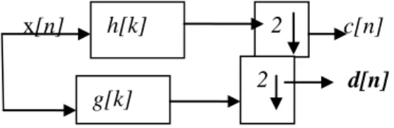
Where the wavelet coefficients g(k) = (-1)^k h(1 - k). Several different sets of coefficients h(k) can be found, which are used to build a unique and or orthonormal wavelet basis. The wavelet transform represents the decomposition of a function into a family of wavelet functions (t) where m is the scale/dilation index and n the time/space index). In other words, using the wavelet transform. Any arbitrary function can be written as a superposition of wavelets. Many constructions of wavelets have been introduced in mathematical and signal processing literature in the context of quadrature mirror filters). In the mid-eighties, the introduction of multiresolution analysis and the fast wavelet transform by Mallat and Meyer provided the connection between the two approaches. The wavelet transform may be seen as a filter bank and illustrated as follows, on a one-dimensional signal x[n]:
•x[n] is high-pass und low-pass filtered, producing two signals d[n] (detail) and c[n] (coarse approximation).
• d[n] and c[n] may be subsampled (decimated by 2: ꜜ2) otherwise the transform is called translation invariant wavelet transform
• the process is iterated on the low-pass signal c[n]. This process is illustrated in Figure 1. We have extract images, the filtering operations are both per-formed on rows and columns, leading to the decomposition.
x[n] c[n]
d[n]
Figure 1. Two-channel filter bank involving subsampling
C.The Least Squares Estimation Method The method of least squares is a standard approach to the approximate solution of overdetermined systems, i.e. sets of equations in which there are more equations than unknowns. "Least squares" means that the overall solution minimizes the sum of the squares of the errors made in solving every single equation [6], [10].
The most important application is in data fitting. The best fit in the least-squares sense minimizes the sum of squared residuals, a residual being the difference between an observed value and the fitted value provided by a model.
Least squares problems fall into two categories: linear least squares and nonlinear
least squares, depending on whether or not the residuals are linear in all unknowns. The linear least-squares problem occurs in statistical regression analysis; it has a closed-form solution. The non-linear problem has no closed solution and is usually solved by iterative refinement: at each iteration, the system is approximated by a linear one, thus the core calculation is similar in both cases.
The least-squares method was first described by Carl Friedrich Gauss around 1794 [8]. Least squares correspond to the maximum likelihood criterion if the experimental errors have a normal distribution and can also be derived as a method of moments estimator.
The objective consists of adjusting the parameters of a model function to best fit a data set. A simple data set consists of n points (data pairs) (xi,yi),i=1,...., n, where I is an independent variable, and Y is a dependent variable whose value is found by observation. The model function has the form f(x, β), where them adjustable parameters are held in the vector ẞ. The goal is to find the parameter values for the model which “host” fits the data. The least-squares method finds its optimum when the sum S of squared residuals is a minimum (equation (5) below).
n
S=∑ ri^2 (5) i=1
A residual is defined as the difference between the value predicted by the model and the actual value of the dependent variable
ri = f(xi, β) - yi. (6) An example of a model is that of the straight line. Denoting the intercept as ᵦo and the slope as ᵦ1, the model function is given by f(x.ᵦ) = ᵦ0 + ᵦ1x. A data point may consist of more than one independent variable. For example, when fitting a plane to a set of height measurements, the plane is a function of two independent
In the most general case, there may be one or more independent variables X and Z and one or more dependent variables at each data point. The minimum of the sum of squares is found by setting the gradient to zero. Since the model contains m parameters there are m gradient equations: ᵩS/ᵩᵦj=2∑ri(∂ri/∂ᵦj)=0,j=1,…,m …..(7) i 2 h[k] 2 g[k]
and since ri=yi-ᶋ(xi, ᵦ) the gradient equations become:
-2∑/ ∂ᶋ(xi, ᵦ)/ ∂ᵦj ri=0, j=1,…….m (8) D. Linear Least Squares
A regression model is a linear one when the model comprises a linear combination of the parameters [6], [10], [12]., i.e.
m
ᶋ(xi,ᵦ)=∑ᵦjᶲj(xi) (9) j=1
where the coefficient, o, are functions of xi. Letting
Xij= ∂ᶋ(xi, ᵦ)/ ∂ᵦj=ᶿj(xi) (10) We can then see that in that use the least-squares estimate (or estimator, in the context of random samples) is given by
ᵦ=(x^T)^-1*X^Ty (11) A generalization to approximation of a data set is the approximation of a function by a sum of other functions, usually an orthogonal set: ᶋ(x) ͇͠ ᶋn(x)=a1ᶲ1(x) + a2ᶲ2(x) +……
+ anᶲn(x) (12)
with the set of functions {ᶲj(x)} an orthonormal set for interest, say [a, b]. The coefficients {aj} are selected to make the magnitude of the difference ||f -f'n ||2 as small as possible.
E. Non-Linear Least Squares
There is no closed-form solution to a non-linear least-squares problem [6]. Instead, numerical algorithms are used to find the value of the parameters ᵦB that minimize the objective. Most algorithms involve choosing initial values for the parameters. Then, the parameters are refined iteratively, that is, the values are obtained by successive approximation.
k+1 k
ᵦj = ᵦj + ∆ ᵦj (13) where k is an iteration number and the vector of increments. ∆ ᵦj is known as the shift vector: In some commonly used algorithms, at each iteration, the model may be linearized by approximation to a first-order Taylor series expansion about ᵦ ^k.
k k
ᶋ(xi,ᵦ)=ᶋ(xi,ᵦ)+∑(∂ᶋ(xi,ᵦ)/∂ᵦj)(ᵦj- ᵦj) (14) The Jacobian J is a function of constants, the independent variable, and the parameters, so it changes from one iteration to the next. The residuals are given by
k m
ri= yi - ᶋ(xi,ᵦ)-∑Jij∆ ᵦj=∆yi-∑Jij∆ ᵦj . (15) To minimize the sum of squares of ri, the gradient equation is set to zero and solved for ∆ ᵦj :
-2∑Jij (∆yi - ∑ Jij∆ ᵦj) = 0 i=1 (16)
j=1 Example:
The methods of least squares and regression analysis are conceptually different. However, the method of least squares is often used to generate estimators and other statistics in regression analysis. Consider a simple example drawn from physics. A spring should obey Hooke's law, which states that the extension of a spring is proportional to the force F applied to it.
Ϝ (Fi, k) =kFi (17) It constitutes the model, where F is the independent variable. To estimate the force constant k, a series of n measurements with different forces will produce a set of data, (Fi. yi.), 1 = 1, where yi is a measured spring extension. Each experimental observation will contain some degree of error. If we denote this error ϵ we may be able to specify an empirical model for our observations
yi = kFi + ϵi (18) There are many methods we might use to estimate the unknown parameter k. Noting that the n equations in the m variables in our data comprise an overdetermined system with one unknown quantity and n e equation. to estimate k may involve using the fewest squares. The sum of squares to be minimized is:
n
S = ∑(yi-kFi)^2 (19) i =1
The fewest squares estimate of the force of the constant k is given by
Ⱪ = (∑iFiyi) / (∑iFi^2) (20) Here, it is assumed that the application of force causes the spring to expand, and having derived the force constant by least-squares fitting, the spring’s extension can be predicted using Hooke's law.
F. A Multi-layered Neural Network Based On Multi-Valued Neurons
A multi-layered neural network based on multi-valued neurons (MLMVNs) has been introduced, investigated, and developed [7], [11], [13]. This network consists of multi-valued neurons (MVNs).that is a neuron with complex-valued weights, and an activation function is defined as a function of the argument of a weighted sum. This activation function was proposed in 1971 in the pioneering paper of N. Aizenberg et al. The multi-valued neurons were introduced based on the principles of multiple-valued threshold logic concerning the field of complex numbers formulated.
The most important properties of MVN are the complex-valued weights, inputs, and outputs lying on the unit circle, and the activation function, which maps the complex plane into the unit circle. The MVN learning algorithm must be reduced to the movement along the unit circle. The MVN learning algorithm is based on a simple linear error correction rule, and it does not require differentiability of the activation function. Different applications of MVNs have been considered during recent years. For example, MVN as a basic neuron in the cellular neural networks; as a basic neuron of neural-based associative memories; as a basic neuron in a variety of pattern recognition systems; and as a basic neuron of the MLMVN.
The MLMVN outperforms a classic multilayer feedforward network, and different kernel-based networks in the terms of learning speed, network complexity, and classification/prediction rates tested for such popular benchmarks problems as the parity n, the two spirals, the sonar, and the Mackey–Glass time series prediction. These properties of MLMVNs show that they are more flexible, and they adapt faster in comparison with other solutions. In this paper, we apply MLMVNs to identify blur and its parameters, which is a core issue in image deblurring.
Usually, blur refers to the low-pass distortions introduced onto an image. It can be caused e.g., by the relative motion between the camera and the original scene, by the optical system, which is out of focus, by atmospheric turbulence (optical
satellite imaging), aberrations in the optical system, etc. Any type of blur, which is spatially invariant, can be expressed by the convolution kernel in the integral equation. Hence, deblurring (restoration) of a blurred image is an ill-posed inverse problem, and regularization is commonly used when solving this problem.
There is a variety of sophisticated and efficient deblurring techniques such as deconvolution based on the Wiener filter, nonparametric image deblurring using local polynomial approximation with spatially-adaptive scale selection based on the intersection of confidence intervals rule. Fourier-wavelet regularized deconvolution, the expectation-maximization algorithm for wavelet-based image deconvolution, etc. All these techniques assume prior knowledge of the blurring kernel or its point spread function (PSF) and its parameter.
When the blurring operator is unknown, the image restoration becomes a blind deconvolution problem. Most of the methods to solve it are iterative, and, therefore, they are computationally costly. Due to the presence of noise, they suffer from stability and convergence problems.
The original solutions of blur identification problems that are based on the use of MVN-based neural networks were proposed in [7]. Two different single-layer MYN based networks have been used to identify blur and its parameter (e.... variation for the Gaussian blur, extent for motion blur, etc.). The results were good, but this approach had some disadvantages. For instance, the networks used have a specific architecture with no universal learning algorithm, thus each neuron was trained separately. Another disadvantage is the use of too many spectral coefficients as features (a quarter of image size). Thus the learning process was heavy.
A single neural network (the discrete-valued MLMVN) with the original backpropagation training scheme was used to identify both the smoothing operator and its parameter on a single observed noisy image. However, the discrete-valued MLMVN had such a drawback as discrete inputs which result in the quantization error of pattern vectors.
G. Multilayer Neural Network Based On Multi-Valued Neurons
A continuous-valued MVN has been introduced in [7]. It performs a mapping between inputs and a single output using n+1 complex-valued weights
where X =x1,…..,.xn is a vector of complex-valued inputs (a pattern vector) and W = Wo,Wi ...Wn is a weighting vector. P is the activation function of the neuron:
P(Z)exp(i(argZ))=e^Argz=Z/│Z│ (22) Where Z = Wo + Wi Xi + ... W, X, is a weighted sum, arg z is an argument of the complex number z. Arg z is the main value of the argument of the complex number z and z is its modulo The MVN learning is reduced to the movement along the unit circle. This movement does not require differentiability of the activation function. Any direction along the circle always leads to the target. The shortest way of this movement is completely determined by an error that is a difference between the desired and actual outputs. The corresponding leaming rule is:
q i Argz
Wr+1=Wr + (Cr/(n+1))(₤ -℮) X=Wr +( Cr/(n+1))*
₤ - Z/│Z│ X (23)
where I denotes vector with the complex-conjugated elements to input pattern vector X; Wr is a current weighting vector; W is a weighting vector after correction; C is a learning rate. A modified learning rule is:
Wr+1=Wr+Cr/(n+1)│Zr│₤-(Z/│Z│)X (24)
where Zr is a current value of the weighted sum. A multilayer feedforward neural network based on multi-valued neurons (MLMVN) has been proposed. It refers to the basic principles of the network with a feedforward dataflow through nodes proposed by D. E. Rumelhart and J. L. McClelland. The most important is that there is a full connection between the consecutive layers (the outputs of neurons from the preceding layer are connected with the corresponding inputs of neurons from the following layer). The network contains one input layer, m-1 hidden layers, and one output layer. Let us use here the following notations. Let km 7 be a desired output of the 4th neuron from m (output) layer: It will be an actual output of k neuron from the o-th (output) laver. Then the global error of the network taken from the neuron of mh (output) layer is calculated as follows:
όkm = Tkm – ykm (25) th
The square error functional for the S pattern Xs = X1,…..Xn is as follows:
* 2
Es = ∑ (όkm ) (W) (26) where ό is a global error taken from k neuron of m (output) layer, E is a square error of the network for the pattern, and W denotes all the weighting vectors of all the neurons of the network. The mean square error functional for the network is defined as follows:
N
E= (1/N)∑ Es (27) K
where N is the total number of patterns in the training set. The backpropagation learning algorithm for the MLMVN was used; the errors of all the neurons from the network are determined by the global errors of the network (Eqn.25). Finally, the MLMVN leaming is based on the minimization of the error functional (Egn.27). Fundamentally, the global error of the network consists not only of the output neurons errors but of the local error of the output neurons and hidden neurons. It means that to obtain the local errors for all neurons, the global error must be shared among these neurons.
H. The Proposed Least Squares Interpolation Filter
In this section, the Least Square Filter Design will be explained. This filter was proposed to repaint the image depending on the least square calculation method. The result obtained from this filter will be used to remove or reduce the blurring in the blurred images. The main equation of this proposed filter is developed to Eqns. (5) and (6) applied to the suggested mask. The least-square developed equation is:
In this section, the least square filter design will explain. This filter was proposed to repaint images depend on the least square calculation method. The result from this filter will be used to remove or reduce the blurring in the blurred images. The main equation of this proposed filter is developed by Eqns. 5 and 6 applied to the suggested mask. The Leas square developed equation are:
S - ∑ri^2
ri = ((f(xi) - yi) +(M-Yi))/2 ...(28)
where M is the average pixels for the suggested mask
The least-squares interpolation resulted in values that were used to replace the selected pixels in the original image depend on the net of
the neighbor's pixels effect. The replacing operation will cover all pixels on the suggested mask.
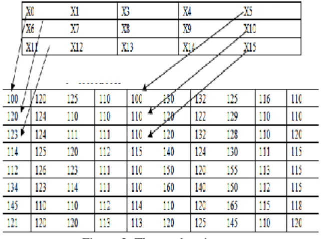
The suggested mask design gives the best pixels effect calculation. The suggested mask contains three rows of 5 image pixels (3x5). Figure (2) shows an example of the design mask. The mask will apply to the whole image until the deblurring operation complete.
Figure 2. The mask points
As shown in Fig.2, the mask points to selected named by x0, x1, x2, x3, ...x15. These selected pixels will be replaced by the resulted values from the Least Square calculation. (Note: the replacing operation will control by the MLMVN network).
I. The Proposed Image Deblurring System Restoration or deblurring average blur from images is a very difficult problem to resolve. In this research, we describe a strategy that can be used for solving such image blurring problems. This strategy is used to evaluate the proposed filter to deblur image control by neural network. The structure of the neural network used in this proposed system was explained bellow.
The proposed filter was designed using the principles and theory of the Least polynomial interpolation to estimate the pixels values to replace in the mask window of the filter.
The operation of the proposed is as shown: firstly, the proposed system applied the wavelet transform(the wavelet transform used is the Daubechies 4D basis wavelet functions applied on the loaded image) on the loaded image. Then select the details sub hand (LL sub-band) to applied the deblurring operation. Second, for each mask window, the proposed system will use the MLMVN to test each pixel in the window if pixel blur or no blur. The MLMVN network was learned to cover three types of the blurred (Gaussian, rectangular, and the motion linear
uniform horizontal). In this proposed system, we used the continuous-valued MLMVN (further simply MLMVN) describe in [7] to solve both the blur and its parameters identification problems in order to overcome the disadvantages mentioned above. The modification of the MLMVN results in significant improvement of the functionality.
At the same time, the proposed system applied the proposed Least-Square Filter to calculate the new replacement pixels values. If the pixel is assigned as a blur with the blur type, the proposed system will replace the pixel by the proposed filter result. Else, the pixel will leave without replacement. The proposed filter and MLMVN network will apply to the whole image. Finally, the proposed system recomposes the resulted image and calculates the RMSE measure to check the variation between the original image and the resulted image.
The main proposed system steps are as follows:
- Apply Wavelet Transform on the loaded image using Daubechies 4D basis function, then, a window of 3x5 coefficients blocks for each sub-bands was used;
-Apply MLMVN neural network on the decomposed image mask;
-Apply adaptive Least-Square Filter on the decomposed image mask;
- IF MLMVN decision id blur replaces with the result of the proposed Least-Square Filter;
- Recompose the deblurred image subbands; - Calculate RMSE
Figure 3 shows the block diagram of the proposed system block:
Figure 3. The block diagram of the proposed system block
In this proposed system, the Daubechies 4D basis filter was used to decomposed loaded image into 2 level using the Daubechies 4D scaling and wavelet functions are as shown in Eqns. (29), (30). Figure 4 shows some results of the 2 levels decomposed image.
ᾳ1= 1+√3∕4√2, α2= 3+√3 ∕4√2
α3= 3-√3 ∕ 4√2, α4 = 1-√3 ∕4√2 (29) β1= 1-√3 ∕ 4√2 , β2=√3 – 3 ∕4√2
β3= 3+√3 /4√2 , β4= -1-√3 /4√2 (30)
Figure 4. Examples of the Daubechies 4D basis filter (2- level).
RMSE can be calculated by :
RMSE=√ n-1 n-1 Z ∑x=0∑Y=0 x(x,y)-(x,y) (31) J. MLMVN Neural Network Structure
As mentioned, the MLMVN network used in the proposed system was explained in [7]. However, we amended the system in terms of the number of input nodes and the blurring types to increase the mask design properties and the performance of the neural network. In this proposed system, we taught the neural network with the three types of the blur with the following parameters. Gaussian blur was considered with
ʈ ϵ {1,1.33 ,1.66, 2, 2.33.2.66,3) for
v(ʈ) = 1/2πʈ^2exp(-((t1^2+t2^2)/(t^2)). (32) where ʈ is a parameter of the PSF (the variance of the Gaussian function). The linear uniform horizontal o = 0 motion blur of lengths 3, 5, 7, 9, for
v(ʈ) = 1/h, √t1^2+t2^2‹h/2,t1 cosᶲ= t2 sin ᶲ 0 otherwise. (33) The rectangular blur window has sizes of 3, 55, 727, and 9 x 9, for
v(ʈ) =. 1/h^2, │t1│‹ h/2 , │t2│‹ h/2
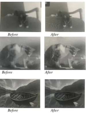
0 otherwise . (34) where parameter h defines the size of the smoothing area. Before After Before After Before After
Fig.(5) Some results of the proposed Least-Square Filter.
The MLMVN has two hidden layers consisting of 5 and 35 neurons and the output layer, which consists of the same number of neurons as the number of classes, i.e., types of blur. Since we consider three types of blur (Gaussian, rectangular, and the motion linear uniform horizontal, o = 0) the output layer contains three neurons. Therefore, the structure
Table 1.
RMSE Results from applies the proposed least square filter
of the network is 15, 5, 35, 3 (input layer, hidden layers, hidden layer 2, output layer). Each neural element of the output layer has to classify a parameter of the corresponding type of blur and reject other blurs (as well as an unblurred image). The MVN activation function (Eqn. 22) for the output layer neurons has a specific form: the equal subdomains (non-overlapping sectors) of the complex plane are reserved to classify a particular blur and its parameters and to reject other blurs and deblurred images.
III. R
ESULTS ANDD
ISCUSSIONIn this research, a least square interpolation calculation was used with a multilayer neural network based on multi-valued neurons to deblur
Sample name RMSE Size
S1 31022 640 X480 S2 30.78 600X800 S3 34.67 600X800 S4 32.21 512X512 S5 32.35 512X512 S6 37.54 600X800
images with full or partial blurring. The proposed filter and MLMVN network achieved very good results in removing the full or partial blurring from the experimental images. Also, good RMSE values resulted. Figure 5 shows the results of the proposed system. The RMSEs of the different samples deblurred by the proposed least square filter are compared in Table 1.
A
CKNOWLEDGMENTSWe would like to express thanks especially to: computer science department, college of science and mustansiriyah university (www. uomustansiriyah.edu.iq ), Baghdad- Iraq.
R
EFERENCES[1] JALOBEANU, A., BLANC-FERAUD,
L., EZERUBIA, J. (2013). Satellite image
deblurring using complex wivelet packets.
International. Journal of Computer Vision, 51
(3),
pp.
205-217.
doi:
10.1023/A:1021801918603
[2] JIA, J. (2007). Single image motion
deblurring using transparency. In: 2007 IEEE
Conference on Computer Vision and Pattern
Recognition, Minneapolis, June 17-22, 2007.
Minneapolis, Minnesota: IEEE, pp.1-8. doi:
10.1109/CVPR.2007.383029