衝突噴流群の流動および熱伝達特性: 沖縄地域学リポジトリ

Title

衝突噴流群の流動および熱伝達特性

Author(s)

Matsuda, Shoichi; Ishiuchi, Toru; Oyakawa, Kenyu

Citation

沖縄工業高等専門学校紀要 = Bulletin of Okinawa National

_{College of Technology(3): 67-76}

Issue Date

2009-03

URL

http://hdl.handle.net/20.500.12001/18665

衝突噴流群の流動および熱伝達特性

松田昇一

機械システム工学科

概要

衝突噴流群は広範囲に大きな熱伝達率が得られることから，ガスタービン翼の冷却および燃焼室の冷却

など工業的に広く利用されている．高温鋼板やシートの冷却では，大きな熱伝達率が必要と同時に一様

に冷却することも重要となる．しかしながら衝突噴流群の流れ場は，隣接する噴流同士の干渉や，壁面

に衝突後外部へ流出する流れとの干渉により複雑となっており，場所によっては，熱伝達率値に大きな

差異がみられる．また最近の機器の小型化に伴い，衝突噴流群も狭い空間内で使用される．その場合，

衝突噴流群の流れ場は隣接する壁面の影響により，さらに複雑な流れ場となり，温度場も複雑となる．

本研究では，比較的狭い空間内において衝突噴流群を垂直に高温壁に衝突させた場合の流れ場と高温壁

面上の温度分布を測定し，流れ場が温度場に及ぼす影響を明らかにすることを目的としている．

流れ場は，噴口上流部より煙を流入させ，噴口と衝突平板間に側面よりシート光（レーザ）を入射し可

視化を行った．煙の粒子径は約 1μm であり，レーザーは出力が 1000mW のグリーンレーザである．

温度場は，衝突平板裏面より赤外線放射温度計を用いて測定を行った．赤外線放射温度計には 256×236

のインジウムアンチモンセンサーが搭載されており，伝熱面全面の温度分布を同時に測定することがで

きる．空間分解能は本実験条件において 0.3×0.3mm であり，フレーム速度は 1/120fps である．

これらの実験結果より，衝突噴流群を垂直に高温壁に衝突させた場合の流れ場が温度場に与える影響を

明らかにし，幾つかの実験式を提案した．

Int. Conf. on Jets, Wakes and Separated Flows, September 16-19, 2008,

Technical University of Berlin, Berlin, Germany

HEAT TRANSFER AND FLOW OF SEMI CONFINED MULTIPLE

IMPINGEMENT JETS

Shoichi Matsuda*

1

, Toru Ishiuchi

2

and Kenyu Oyakawa

2

1

Department of Mechanical Systems Engineering Okinawa National College of Technology,

Nago, Okinawa, Japan E-mail: [email protected]

2

Department of Mechanical Systems Engineering University of the Ryukyus,

Nishihara, Okinawa, Japan

ABSTRACT

This paper shows the influence of flow behavior of multiple impingement jets on characteristics of heat transfer of narrow spaces. The jets were set a 11×11 nozzles of sharp edged orifice type with D=1 mm in diameter. The jet-to-jet space is 4mm. The experiments were performed for the separation distance, H, between jet exit and impingement plate ranging from H/D=5 to 10, at Reynolds number 310 ~ 630.

The time and spatial temperature profiles over the impingement plate were measured using an infrared camera (TVS-8500, Avio) with a two-dimensional array of Indeum-Antimony (In Sb) sensors.

To clarify the influence of the flow behavior on heat transfer fields, we visualized a smoke flow field by means of a laser light sheet method (LLS).

Based on these experimental data, the relationships between the fluid flow and the heat transfer characteristics were clarified.

1. INTRODUCTION

Impingement jets have been widely used for rapidly cooling and heating the surface or a body in engineering because relatively high heat transfer coefficients are obtained near the stagnation point of the impingement plate on which the jet impinges. Another advantage is that heat-loads on the surface can be easily controlled since the local heat transfer coefficients over the plate have been nearly estimated when the diameter of the nozzle exit issuing jet and the separation distance between the nozzle exit and the plate are known.

The cooling of the heated surface which is elements of gas turbine blades or combustion chambers has not been achieved with single jet but by using multiple jets which eject the fluid flow in a staggered or square fashion. Multiple impingement jets has the advantage that the high heat transfer coefficients can be obtained in wide area. Mori et al.(1) experimentally investigated heat transfer characteristics on a plate of multiple jets by varying the arrangement of the jets and the protrusion on the plate in order to improve the heat transfer characteristics, when two-dimensional multiple jets impinged on a heated surface with roughness.

When a high temperature steel slab is cooled or a thin film is dried by multiple jets flow, it becomes very important to heat or cool the surface uniformly, and to enhance the heat transfer coefficients simultaneously. Multiple jets were used in certain arrangements in order to get high and uniform heat transfer coefficients; and its feature is different from a single jet. When the jet-to-jet space and the separation distances between nozzle exit and plate distance are small, the adjoining jets may interfere with each other before the

jets attached to the target plate. In the present study (2), (3), when the jet-to-jet space is L/D=2 and the separation distances between nozzle exit and plate is H/D=2, the neighboring jets unite before it attaches to the target plate. This display looks like that of the elliptic jet having the axes-switching phenomena observed generally on a non-circular jet. When the target plate was placed sufficiently far downstream from the exits, the jets behave the same as that of the single jet. Thus both space jet-to-jet and separation between jet exit and the plate are the most important parameters in considering interference phenomena of multiple jets. Furthermore, the multiple jets are affected by the spent flow streamed downstream direction after the jet impinged. Therefore, the heat transfer coefficient may be lower than that the single impingement jet due to the interference of the adjoining jets and the spent flow. Obot and Trabold(4) investigated how heat transfer was affected by the spent flow of the jets being issued from circular orifice nozzles and successively impinged over a heating surface, then being dispersed outward; this was done in a rectangular passage with a two or three dimensional flow field.

Recently, accompanying the miniaturization of the equipment, multiple jets have been applied in narrow spaces. In this case, heat and flow behavior of multiple jets show more complicated characteristics due to the increase of the interactions between adjoining jets, furthermore between jet and spent flow. Bertrand P.E.et al. (5) experimentally investigated the heat transfer characteristics of multiple jets with a narrow space. They clarified heat transfer characteristics at the large range of Reynolds number when the multiple impingement jets impinged to the target plate in narrow spaces. However, the influence of the flow behavior gives on heat transfer fields is not yet clear.

In this paper, to make clear the effect of the flow behavior on heat transfer fields, the time and spatial temperature profiles over the impingement plate were measured using an infrared camera (TVS-8500, Avio) with a two-dimensional array of Indeum-Antimony (In Sb) sensors when jets being issued from a multiple nozzle impinge on the target plate. At the same time, a smoke flow field was visualized by means of a laser light sheet method (LLS), for the multiple jets formed 11×11 arrays in a lattice pattern, where the diameter of jets was 1mm and the jet-to-jet space is 4 mm.

The heat transfer mechanism was discussed based on these results obtained flow and temperature fields. In addition to these results, the relation among the averaged Nusselt number, Reynolds number and separation distances between nozzle exit and the plate was proposed as the experimental equation.

NOMENCLATURE

D: diameter of nozzle [mm]

H: distance between jet exit and impingement plate [mm] hx: local heat transfer coefficient [W/m2K]

L: distance between nozzle [mm]

Nu: Nusselt number (=hx D/λ)

q: heat flux on the plate [W/m2]

Re: Reynolds number (=U0 D/ν)

tj : temperature of jets at the nozzle exit [K]

tw : wall temperature [K]

U0 :jet velocity at nozzle exits [m/s]

X: coordinate of horizontal direction in figure Y: coordinate of vertical direction in figure

Greek symbol

λ : Thermal conductivity of working fluid [W/mK]

ν : Kinematic viscosity of working fluid [m2

/s]

2. EXPERIMENTAL SETUP AND

PROCEDURE

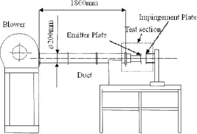
Figure 1 shows the schematic diagram of the experimental apparatus. The experiments were carried out in a specially designed open circuit wind tunnel having a jet emitter at the end. Air was supplied to the jet emitter with a nozzle by a blower with variable speed controlled through a calibrated orifice as a working fluid.

The arrangement of the nozzle, impingement plate, infrared camera, and some dimensions are shown also in Fig.2. The multiple jets issuing from the emitter plate of multiple nozzles were struck onto a vertical target plate.

Detail of the emitter plate and some dimensions is shown in Fig. 3. The emitter plate is 5mm thick, 150mm high and 150mm wide of polished aluminum plate, was drilled to 1mm diametric orifice holes in central portion. The multiple jets are formed in 11×11 arrays in a lattice pattern. The jet-to-jet space is 4mm, and thus ratio of it to diameter is L/D=4. The origin point is at center of the jet exits located in the center portion of the emitter plate, lateral direction from origin point is X and the vertical direction is Y as shown in Fig. 3.

The impingement plate was made of a Bakelite plate 150mm high, 150mm wide, and 10mm in thickness as shown in Fig.4. The stainless steel foil of 10µm in thickness (180mm×100mm) was attached to the impingement plate as the heating surface. This keeps a constant heat flux by supplying a direct current.

The temperature distribution over the heating surface was measured by means of the infrared camera while observing the thermo image of the back of the stainless steel foil through the window of 50mm high and 50mm wide at the center portion on the impingement plate as shown in Fig 4. It is located in back of the heating stainless steel foil in order to observe the temperature distribution of the heating surface. This is due to the fact that the heating surface temperature was considered to be same as that of the back surface because the thickness of stainless steel foil was very thin; 10µm. The back of the stainless-steel foil was painted black in order to measure temperature distribution with a high level of accuracy.

Fig.2 Arrangement of Nozzle, impingement plate

and infrared camera

Fig.3 Detail of multiple nozzle

Fig.1 Schematic diagram of the experimental

apparatus

Poly vinylidene chloride film which has a transmissivity for infrared energy at near unity was attached to the back of impingement plate to cover the window, and to prevent heat dissipation from the back of the heating surface. The temperature resolving power of the infrared camera is 0.025 K on a black body and an infrared camera scans the thermo-images at 256×236 points on the heating surface per 1/120 second with 0.05 K sensitivity. The spatial resolving power is 0.3×0.3mm per one element when the distance between heating surface and infrared camera is 30cm. Measurement waves length are 3.5 to 4.4mm and 4.5 to 5.1mm.

The heat transfer coefficients were calculated using hx=q/(tw-tj ),

where q is the heat flux on the plate, tw is the wall temperature

measured by the infrared image, and tj is the temperature of the jets

measured by T type thermocouples of 70µm diameter inserted into the jet exit. The infrared camera cannot catch the real temperature of the surface of the impingement plate because its surface is not a black body, and infrared energy does not completely penetrate the poly vinylidene film. Therefore, the temperature measured by the infrared image was calibrated by using a thermocouple soldered onto the stainless steel foil, as shown in Fig.4.

To know the flow behavior of the multiple impingement jets, we visualized a smoke flow field by means of a laser light sheet method (LLS). The diameter of the smoke particles are approximately between 0.3 to 1 µm. Laser light sheet is a green laser (Nd/YVO4, 53nm) which power is 1000mW. Width of the

Laser Light Sheet is 0.7 mm at a distance of 1m away from laser exit. The smoke particles were inserted from the upstream region of the nozzle exits and it is exhausted through each nozzle jets, after that it impinged to the target plate. Laser light sheet was irradiated between the emitter plate and the target plate shown as Fig. 5. And we caught a picture of smoke flow from the vertical direction to the laser light sheet by using the high speed video camera. The maximal frame rate for this high speed video is 130,000fps.

The experiments were done at a nozzle exit velocity between 5m/s and 10m/s, and the corresponding Reynolds number was between 300 and 630 based on the nozzle diameter and a nozzle exit velocity. The jets impinged to the impingement plate for various distance from jet exit to the impingement plate.

3. RESULTS AND DISCUSSION

3.1 Flow characteristics of the multiple

impingement jets

The flow behavior of multiple jets show complicated characteristics due to the existence of the interactions between adjoining jets, in addition, between jets and spent flow. In order to clarify the influence of the flow behavior on heat transfer fields, we visualized a smoke flow when the multiple jets impinged on the target plate. A visualized flow at H/D=5 and H/D=10 are shown in Fig.6 (a) and (b), respectively. Reynolds number of jet is 310, and the frame rate of the high speed camera is 100 fps. The longitudinal and abscissa axes show Y/D and H/D, respectively. The left side and the right side in the figure are corresponded to the jets exit and the impingement plate, respectively. Y/D=0, ±4, ±8, ±12 and ±16 correspond to the center of the nozzle exits. Green part in Fig.5 shows the tracer particle. The bottom in the figure looks darker

than upper side, because the laser was irradiated between the emitter plate and impingement plate from the upper side as shown in Fig.5. At H/D=5 shown in Fig.6(a), the jets from the jets emitter impinged vertically to the impingement plate and then flowed to a radial direction along the impingement plate as the spent flows. Near the impingement plate, we can see the vortex that looks like a small black area in the figure. At the outer portion, both spent flows and the vortex prevent the jets from impinging to the target plate and the jet flows are bent to a radial direction. In addition, the position of the vortex near the plate gradually moves to the outer portion, and thus the impingement point gradually moves to the outer portion. At H/D=10 shown in Fig.6 (b), each jets vertically impinged to the impingement plate, and we can see the vortex in Y/D=0, ±4, ±8, ±12 and ±16 neighborhood near the plate similar to that of H/D=5.

To see a detailed flow field, the flow field where the center portion in Fig. 6 was expanded as like shown in Fig. 7. The arrow in Fig.7 shows the direction of the flow. At H/D=5 shown in Fig.7 (a), after the jets flow impinged, a spend flow along the plate from

Y/D=0 collides with a spend flow along the plate from Y/D=±4 on

vicinity of the middle of Y/D=0 and Y/D=±4. After that the flows separate from the impingement plate and then flow upstream region toward the emitter plate direction. The flows to the upstream region impinge to the emitter plate and then flow to a radial direction

Fig.5 Schematic diagram of the experimental apparatus

for flow visualization

along the emitter plate. Finally, these flows entrained to the neighborhood of the main jet flows and impinged the impingement plate again. Like this, the circulating flows are generated between the main jets flows. At H/D=10 shown in Fig.7 (b), the flow to the emitter plate was created by the spent flows between the jets. After that it was entrained by the neighborhood jets. It differs from the case of H/D=5, the flows do not reach the emitter plate. At H/D=5 and H/D=10, the circulation flows between the jets formed two vortexes in a mutually opposite direction. These vortexes interfered with the jet and caused a change in the flow of direction.

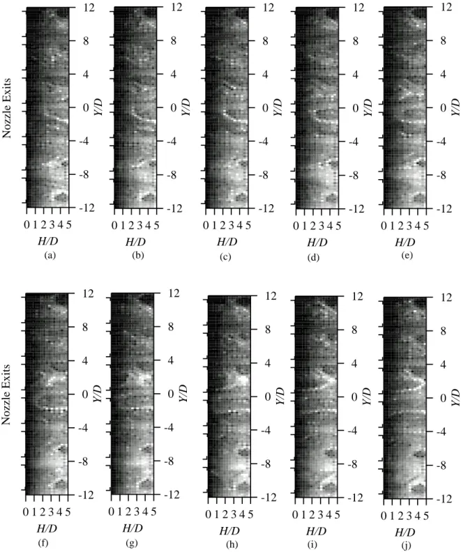
From these results, the appearance of a time average flow field was understood. An actual flow field greatly changes in time. In order to realize the instantaneous flow field, Fig. 8 (a) ~ (j) shows the instantaneous flow field with the frame rate of the high speed camera is 1000 fps. Overall, the jets and the spend flows change along with time in Fig.8. Pay attention to the flow from the impingement plate to the jets emitter plate at Y/D=-2 in Fig.8 (a). While advancing from Fig.8 (a) to Fig.8 (d), this flow direction is gradually inclined to an upward direction in figure. While proceeding from Fig.8 (e) to Fig.8 (g), this flow direction is gradually returned to the original direction that is vertical to the impingement plate. While advancing from Fig.8 (h) to Fig.8 (j), this flow direction is gradually inclined to a downward direction. The cycle period of this flow cycle changes about 0.01 seconds.

3.2 Isotherms of infrared images

The time averaged heat transfer coefficients hx are calculated by using thermal data from the infrared images. Figure 9 (a) and (b) shows the time averaged heat transfer coefficients on the impingement plate at H/D=5 and H/D=10 for Re=310. This figure shows an averaged value of heat transfer in about 0.1 seconds. Here, to make an easier comparison on the other parameter, the value in which the local heat transfer is divided by the maximum heat transfer in Fig.9 and 10 are indicated. The red color region in Fig.9 and 10 show the high heat transfer part and a blue color region in Fig.9 and 10 show the low heat transfer part. At H/D=5 shown in Fig.9 (a), the high heat transfer coefficients regions for the center portion are almost coincident with the position of nozzle exit. Thus, this result is corresponding to the jets vertically impinged to the impingement plate. For the outer portion, the high heat transfer coefficients regions slightly shift to radial directions. This is due to the jets interference with the spent flow before it reaches the impingement surface and the axis of the jets pressed toward spent flow directions. Thus, the jets flow in the outer portion inclines outside as shown in Fig.6 (a). At H/D=10 shown in Fig.9 (b), the high heat transfer coefficients regions for the center portion and the outer portion are almost coincident with the position of the nozzle exit similar to that of H/D=5. However, the difference between the higher heat transfer regions and lower heat transfer region becomes small and it approaches overall at the same heat transfer coefficients. This is due to the jets impinging to the target plate while developing enough and having extended spatially, comparing with H/D=5. Thus the neighboring jets interfere with each others before the jets reach the impingement plate.

At Fig.9 (a) and (b), comparing the heat transfer coefficients of the upper area with the heat transfer coefficients of the downside area, the heat transfer coefficients of the downside area shows higher

(a) H/D=5

(b) H/D=10

Fig.7 Detail of Flow field

(Frame rate =100fps, Re =310)

Nozzle Exits -4 -3 -2 -1 0 1 2 3 4 5 4 3 2 1 0 H/D -4 -3 -2 -1 0 1 2 3 4 Y/D 10 8 6 4 2 0 H/D

(a) H/D=5 (b)

H/D=10

Fig.6 Visualization of flow

(Frame rate =100fps, Re =310)

Nozzle Exits -16 -12 -8 -4 0 4 8 12 16 5 4 3 2 1 0 H/D -16 -12 -8 -4 0 4 8 12 16 Y/ D 10 8 6 4 2 0 H/D

values than that of the upper area. This phenomenon was caused by the heating surface on downside area to be cooled by natural convection rather than the upper area.

Figure 10 (a) and (b) shows the time averaged heat transfer coefficients on the impingement plate at H/D=5 and H/D=10 for Re=610. At H/D=5 shown in Fig.10 (a), the high heat transfer coefficients regions for the center portion are almost coincident

with the position of nozzle exit similar to that of Re=310. For the outer portion, almost the same as Re=310. Comparing that of

Re=320 with that of Re=610, the difference between the higher heat

transfer region and lower heat transfer region becomes large in the center portion because of increased nozzle exit velocity. At

H/D=10 shown in Fig.10 (b), the difference between the higher

heat transfer region and lower heat transfer region becomes small

No

e

s

-12

-8

-4

0

4

8

12

Y/D

5

4

3

2

1

0

H/D

-12

-8

-4

0

4

8

12

Y/D

5

4

3

2

1

0

H/D

-12

-8

-4

0

4

8

12

Y/

D

5

4

3

2

1

0

H/D

Nozzle Exits

-12

-8

-4

0

4

8

12

Y/D

5

4

3

2

1

0

H/D

-12

-8

-4

0

4

8

12

Y/D

5

4

3

2

1

0

H/D

Fig.8 Instantaneous flow field (frame rate =1000 fps, H/D=5, Re =310)

(a) (b)

_(c)

_(d)

(e)

(f) (g)

(h)

(i)

(j)

Nozzle Exits

-12

-8

-4

0

4

8

12

Y/D

5

4

3

2

1

0

H/D

-12

-8

-4

0

4

8

12

Y/D

5

4

3

2

1

0

H/D

-12

-8

-4

0

4

8

12

Y/D

5

4

3

2

1

0

H/D

-12

-8

-4

0

4

8

12

Y/D

5

4

3

2

1

0

H/D

-12

-8

-4

0

4

8

12

Y/D

5

4

3

2

1

0

H/D

in comparison to the distribution of heat transfer coefficients at

H/D=5.

Instantaneous isotherm images at H/D=5 for Re=310 was shown in Fig.11 (a) and (b). The frame rate of infrared camera is 120 fps.

(b) H/D=10

(a) H/D=5

Fig.11 Instantaneous isotherm of infrared images (Frame rate 120 fps, H/D=5, Re =310)

Fig.9 Time averaged heat transfer on the plate (0.1sec., Re=310)

-24 -20 -16 -12 -8 -4 0 4 8 12 16 20 24 Y/ D -24 -20 -16 -12 -8 -4 0 4 8 12 16 20 24 X/D 1.0 0.8 0.6 0.4 0.2 0.0 -24 -20 -16 -12 -8 -4 0 4 8 12 16 20 24 Y/ D -24 -20 -16 -12 -8 -4 0 4 8 12 16 20 24 X/D 1.0 0.8 0.6 0.4 0.2 0.0 -24 -20 -16 -12 -8 -4 0 4 8 12 16 20 24 Y/ D -24 -20 -16 -12 -8 -4 0 4 8 12 16 20 24 X/D 1.0 0.8 0.6 0.4 0.2 0.0 -24 -20 -16 -12 -8 -4 0 4 8 12 16 20 24 Y/D -24 -20 -16 -12 -8 -4 0 4 8 12 16 20 24 X/D 1.0 0.8 0.6 0.4 0.2 0.0

(b) H/D=10

(a) H/D=5

Fig.10 Time averaged heat transfer on the plate (0.1sec., Re=630)

-24 -20 -16 -12 -8 -4 0 4 8 12 16 20 24 Y/ D -24 -20 -16 -12 -8 -4 0 4 8 12 16 20 24 X/D 80 70 60 50 40 30 -24 -20 -16 -12 -8 -4 0 4 8 12 16 20 24 Y/ D -24 -20 -16 -12 -8 -4 0 4 8 12 16 20 24 X/D 80 70 60 50 40 30

(b)

(a)

The dark blue color in Fig.11 (a) and (b) shows a lower temperature. The lower temperature regions are almost coincident with the position of nozzle exit and that remain independent in Fig. (a). On the other hand, at Fig. (b), the lower temperature region for the center portion is adjoining the neighborhood of the lower temperature region. Since the cycle of the flow change is about 0.01 seconds, the frame rate of infrared camera is not enough to catch these instantaneous phenomena unfortunately. However the difference between the time averaged isotherm and instantaneous isotherm is approximately clear.

3.3 Distribution of heat transfer coefficients

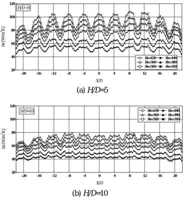
The variation of the local heat transfer coefficient distributions along the X/D with Re =310 ~ 630, at H/D=5 and 10 are shown in Fig. 12 (a) and (b). At H/D=5, the distribution have peaks at the nozzle position. These values of peaks are gradually increased with increasing Reynolds number. The positions of peaks move to the outer portion corresponding to the jets flow in the outer portion which inclines outside as shown in Fig.6 (a). At H/D=10, the distributions are becoming small overall comparing with that of H/D=5. And thus, the difference of the high heat transfer and the low heat transfer is small.

The distributions of the local heat transfer coefficient along the

X/D with Re =310, 630, at H/D=5, 6, 7, 8, 9 and 10 are shown in

Fig. 13 (a). (b). At Re =310, the distribution has peaks at the nozzle exit position. The value of the peak is gradually decreased with increasing H/D. And the positions of the peaks move to the outer portion with increasing H/D. At the lower Reynolds number, the distributions are almost constant. At Re =630, the distribution has peaks at the nozzle exit position and this value of the peaks is gradually decreased with increasing

H/D. This value is larger than that of Re =310.

3.4 Averaged heat transfer characteristics

To obtain the information about heat transfer characteristics, averaged heat transfer was estimated by overall instantaneous temperature distribution which was measured with infrared camera in range of -16≦X/D≦16 and -16≦Y/D≦16. It was averaged within this range to prevent the wall edge of observation window from influencing it.

Figure 14 shows the change of averaged Nusselt number based on averaged heat transfer coefficients and nozzle exit diameter with Reynolds number for various separation distance between nozzle exit and the plate. Nusselt number gradually increases with an increasing Reynolds number at the all H/D and increases with a decreasing in H/D. The highest Nusselt number at H/D=5 depends on 0.69th power of Reynolds number like shown in the equation (1). On the other hand, the lowest Nusselt number at

H/D=10 depends on 0.66th power of Reynolds number shown in

the equation (2). Thus the increase rate of Nusselt number slightly becomes smaller as the H/D becomes larger.

Nu=0.038 Re

0.69

(H/D=5)

(1)

Nu=0.037 Re

0.66

(H/D=10)

(2)

(b) H/D=10

(a) H/D=5

(b) Re=630

Fig.13 Distributions of local heat transfer

coefficient varying separation distance

(a) Re=310

Fig.12 Distributions of local heat transfer

coefficient varying Reynolds number

120 100 80 60 40 20 hx [W /m 2K] -20 -16 -12 -8 -4 0 4 8 12 16 20 X/D Re=630 Re=440 Re=560 Re=380 Re=500 Re=310 H/D =5 120 100 80 60 40 20 hx [W /m 2K] -20 -16 -12 -8 -4 0 4 8 12 16 20 X/D Re=630 Re=440 Re=560 Re=380 Re=500 Re=310 H/D=10 120 100 80 60 40 20 hx [W /m 2K] -20 -16 -12 -8 -4 0 4 8 12 16 20 X/D Re =310 H/D=5 H/D=8 H/D=6 H/D=9 H/D=7 H/D=10 120 100 80 60 40 20 hx [W /m 2K] -20 -16 -12 -8 -4 0 4 8 12 16 20 X/D Re =630 H/D=5 H/D=8 H/D=6 H/D=9 H/D=7 H/D=10

Figure 15 shows the change of averaged Nusselt number with the separation distances between nozzle exit and plate for various Reynolds number. Nusselt numbers gradually decrease with an increasing H/D at the all Reynolds number and decrease with a decreasing in Reynolds number. The highest Nusselt number at

Re=630 depends on -0.33th power of H/D shown in the equation

(3). The lowest Nusselt number at Re=320 depends on -0.26th power of H/D shown in the equation (4). Thus the decrease ratio of

Nusselt number slightly becomes smaller as the Reynolds number becomes smaller.

Nu=5.63 (H/D)

-0.33

(Re=630) (3)

Nu=2.94 (H/D)

-0.26

(Re=320) (4)

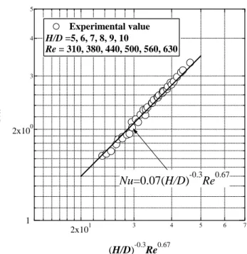
To simplify the experimental equations, the dependency of Nusselt number to Reynolds number is assumed to be Re0.67 and the dependency of Nusselt number to H/D is assumed to be (H/D)-0.3. Here, this dependence of the Reynolds number is similar to that of colliding of the large scale vortex and the colliding of the large shearing flow. In addition, the Nusselt number is arranged by (H/D)-0.3Re0.67. Figure 16 shows the correlation between averaged Nusselt number and (H/D)-0.3 Re0.67. Finally, the Nusselt number is expressed approximately by the equation (5). This equation (5) can be approximated with an error 4.5% or less.

Nu = 0.07(H/D)

-0.3

Re

0.67

(5)

4. CONCLUSIONS

Characteristics of the heat transfer on a plate being impinged by multiple jets were investigated experimentally by visualizing the flow and measuring the isotherms images. The results are:

(1) The jets perpendicularly impinged to the impingement plate and then flow to a radial direction along the impingement plate as the spent flows. For the outer portion, the jets flow are bent to the radial direction because of the interaction of adjoin jets and spent flows.

Fig.14 Variation of averaged Nusselt number

with Reynolds number for various H/D

Fig.15 Variation of averaged Nusselt number

with H/D for various Reynolds number

1 2x100 3 4 5 Nu 2 3 4 5 6 7 8 9 1000 Re H/D=5 H/D=6 H/D=7 H/D=8 H/D=9 H/D=10 1 2x100 3 4 5 Nu 3 4 5 6 7 8 9 10 H/D Re=630 Re=560 Re=500 Re=440 Re=380 Re=310

Fig.16 Characteristics of averaged Nusselt number

1 2x100 3 4 5 Nu 2x101 3 4 5 6 7 (H/D)-0.3Re0.67 Experimental value H/D =5, 6, 7, 8, 9, 10 Re = 310, 380, 440, 500, 560, 630

Nu=0.07(H/D)

-0.3

Re

0.67

(2) For instantaneous flow field, the jets and the spend flows change along with the time. The cycle period of this flow change is about 0.01 seconds.

(3) The high heat transfer coefficients regions for the center portion are almost corresponding to the position of nozzle exit. At the outer portion, that region slightly moves to the radial directions corresponding to the jets flow which inclines outside. The difference between the higher heat transfer region and lower heat transfer region has become small in case of increasing H/D and decreasing Re. And it approaches the same heat transfer coefficients overall.

(4) Instantaneous isotherm images change corresponding to the instantaneous flow field.

(5) The distributions of the local heat transfer coefficient have the peaks at the nozzle position. This value of peaks is gradually increased with increasing Re and with decreasing

H/D. The positions of peaks shift to the outer portion

corresponding to the jets flow which inclines outside. (6) Nusselt number depends nearly on 0.67th power of Reynolds

number and on -0.3th power of H/D. and thus, Nusselt number is arranged by (H/D)-0.3Re0.67 shown in the equation (5). This equation (5) can be approximated with an error 4.5% or less.

References

1. Mori, Y. Uchida Y. Koizumi H., Impinging Cooling of a High Temperature Flat surface by Multiple Two-dimensional Air jets, Trans. JSME B, Vol.54, No.502, pp.1434-1438, 1988

2. Oyakawa K. Matsuda S. Yaga M. Tashiro A., Heat Transfer Characteristics by Impingement Jets Issuing from Dual Elongated Slot Nozzles, Heat transfer, Trans JSME Ser B, Vol.65, No.637, pp.3084-3090, 1999

3. Oyakawa K. Hanashiro K. Matsuda S. Yaga M and Hiwada M., Study on Flow and Heat Transfer of Multiple Impingement Jets, Heat Transfer-Asian Research, 34(7), 2005

4. N.T. Obot, and T.A. Trabold, Impingement Heat Transfer within Arrays of Circular Jets: Part 1-Effects of Minimum, Intermediate, and Complete Crossflow for Small and Large Spacings. J. Heat Transfer, Vol.109, pp.872-879, 1987

5. B.P.E. Dano, J. A. Liburdy, K. Kanokjaruvijit, Flow

Characteristics and Heat Transfer Performances of a Semi-confined Impinging Array of Jets: Effect of Nozzle Geometry, Int. J. Heat Mass Transfer, vol.48,pp.691-701, 2005

Int. Conf. on Jets, Wakes and Separated Flows

September 16-19, 2008, Technical University of Berlin, Berlin, Germany