Chapter 4 The Challenges in Developing
Realistic NEG Simulation Models for East Asia
権利
Copyrights 日本貿易振興機構(ジェトロ)アジア
経済研究所 / Institute of Developing
Economies, Japan External Trade Organization
(IDE-JETRO) http://www.ide.go.jp
journal or
publication title
New Challenges in New Economic Geography
page range
131-156
year
2010-03
131
Kumagai, Satoru, ed. 2010. New Challenges in New Economic Geography.Chiba: Institute of Developing Economies.
Chapter 4 The Challenges in Developing Realistic NEG
Simulation Models for East Asia
Satoru KUMAGAI
*aAbstract
This chapter attempts to identify some important issues in developing realistic simulation models based on new economic geography, and it suggests a direction for solving the difficulties. Specifically, adopting the IDE Geographical Simulation Model (IDE-GSM) as an example, we discuss some problems in developing a realistic simulation model for East Asia. The first and largest problem in this region is the lack of reliable economic datasets at the sub-national level, and this issue needs to be resolved in the long term. However, to deal with the existing situation in the short term, we utilize some techniques to produce more realistic and reliable simulation models. One key compromise is to use a ‘topology’ representation of geography, rather than a ‘mesh’ or ‘grid’ representation or simple ‘straight lines’ connecting each city which are used in many other models. In addition to this, a modal choice model that takes into consideration both money and time costs seems to work well.
Keywords: Geographical Simulation Model, East Asia, spatial economics, modal choice
JEL classification: D59, F29, R49, O53
*a Researcher, Economic Integration Studies Group, Inter-disciplinary Studies Center, IDE
132
1. Introduction
Following the remarkable progress in the theoretical aspects of NEG in the 1990s, some realistic simulation models appeared in the 2000s, although their numerical simulations are rather minor (Fujita and Mori 2005:396-397). There appear to be two strands of studies using NEG-based simulation models. The first one evaluates the effects of a specific policy, mainly transport policy, on the spatial economic structure in a region.1 Teixeira (2006) applied an NEG-based simulation model to evaluate the transport policy in Portugal and concluded that the development of transport networks theretofore had not contributed to the spatial equity in the region. Bosker et al. (2007) divide the EU into 194 NUTS-II level regions and observe the effect of further integration of the EU using a model based on Puga (1999). The authors found that further integration leads to higher levels of agglomeration.
The second strand tests the validity of the NEG theory by comparing the results generated by simulations with actual data. For instance, Fingleton (2006) investigates the validity of the NEG model vis-à-vis the urban economics (UE) model when applied to the spatial wage structure in Great Britain and finds that UE, rather than NEG, possesses more explanatory power. On the other hand, Stelder (2005) tries to replicate the scale and locations of agglomerations in Europe using the NEG model by dividing the region into a grid of 2627 squares. The author concluded that the model explains the locations and scale of the agglomerations to a substantial degree. Bosker et al. (ibid.) also tries to replicate the distribution of the manufacturing labour force in the EU and succeeds fairly well.
The IDE-GSM obviously is affiliated with the first strand of studies, although it displays some variances. The first and most important variance is that the IDE-GSM is intended to evaluate the effects of infrastructure development in the future, not the past. This is solely because there is inadequate time series economic data for the region at the sub-national level in order to evaluate the past infrastructure development projects. Secondly, although many of the studies in this field focus on the EU as an area of study,
1
In research on the EU, several attempts have been made to simulate the effects of infrastructure development using the spatial CGE model, including Bröcker et al. (2004).
133
the IDE-GSM simulates the economic geography of Southeast Asia. There are very few NEG-based models for Southeast Asia, and none of them covers this large area using realistic features. Thirdly, as explained in the following sections, the IDE-GSM incorporates a fairly realistic transport topology and modal choice in the model. This affords a strong advantage when evaluating the effects of a specific transport infrastructure development project.
This chapter is constructed as follows. In Section 2, the base model of the IDE-GSM is concisely explained, and extensions to tailor the simple model to reality are introduced. In Section 3, the three types of geographical representation often used in the NEG model are introduced, and an explanation is presented concerning why the IDE-GSM adopts the ‘topology’ representation. Sections 4 through 7 discuss the specific difficulties encountered when we desire to make the model more realistic. Section 8 states the specifics of the problem particular to East Asia, i.e., the lack of geo-economic data. Finally, the last section concludes this chapter.
2. From the Laboratory to the Real World
2.1 The CP Model in Two Locations
The NEG model, either theoretical or empirical, tends to be complex and difficult to solve mathematically. So, NEG studies frequently use numerical simulation. The very basic model, the core-periphery (CP) model by Krugman (1991) also uses numerical solutions to show the fundamental characteristics of the NEG model. The basic CP model is a two-location-two-goods model, setting one good (typically assumed as an agricultural good) as numeraire, which is produced using constant return to scale technology and incurs zero transport costs, while the other good is produced using increasing return to scale technology (typically assumed as a manufactured good) and incurs some positive transport costs.
Manipulating the CP model, we can understand the basic behavior of the typical NEG model, such as 1) manufacturing activity tends to diverge if the transport costs are very high or very low, 2) manufacturing activity tends to concentrate if the share of the
"$%
income spent on manufactured goods is large and 3) manufacturing activity tends to concentrate if the elasticity of substitution is high, all other things being equal.
2.2 The CP Model in Many Locations
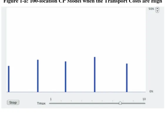
The CP model can be extended to an arbitrary number of locations. Krugman (1993) extends it to 12 locations on the line, connecting both sides, and calls it a ‘racetrack economy.’ In this model, we can explore the relationship between parameters and the number of agglomerations. The typical findings are: 1) The number of agglomerations tends to decrease as the products are more differentiated, 2) The number of agglomerations tends to increase as the share of manufacturing in the consumption expenditure becomes lower and 3) The number of agglomerations tends to increase as the transport costs become higher, all other things being equal. These tendencies are basically retained in the extended simulation model that uses the CP model as a base model.
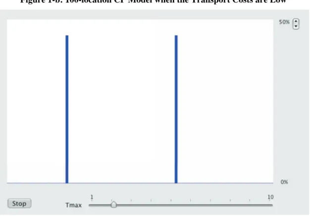
Figures 1-a and 1-b are examples of the equilibrium agglomerations in the higher and lower transport costs settings simulated by the 100-location model.2
Figure 1-a: 100-location CP Model when the Transport Costs are High
2
The model used for Figures 1-a and 1-b is basically identical with that of Krugman (1991), although the number of locations has been expanded from 12 to 100.
"$&
Figure 1-b: 100-location CP Model when the Transport Costs are Low
The beauty of the CP model in many locations is its simplicity and its rich implications that are easily applicable to a real world setting. Indeed, the IDE-GSM was launched as a branch of the CP model featuring many locations, with the difference that the ‘geography’ is not ‘racetrack’ but a realistic topology of the cities.
2.3 Proper Level of Complexity of the Model
The models used in simulation can be far more complex than those used in theoretical analyses because the latter should be as simple as possible to solve mathematically, while the former need not be.
However, a complex model has some disadvantages even in simulation studies. Firstly, a complex model contains more parameters, meaning that these parameters need to be determined properly. For instance, we do not need to cancel out fixed cost in the production function of the manufacturing sector in the CP model when doing a simulation, but if we leave the fixed cost parameter in the model, then we need to specify it. So, the more realistic and complex the model becomes, the more data is needed to establish the parameters properly.
136
Secondly, a complex model tends to yield complex results. Sometimes, it is difficult to interpret the changes in a simulation’s results that occur in response to the changes in the data and parameters when the model which is used becomes complex. So, when we select the base model for use in a simulation, it is important to achieve balance between the realistic nature of the model and the ease of handling and understanding the model.
3. Geographical Representation
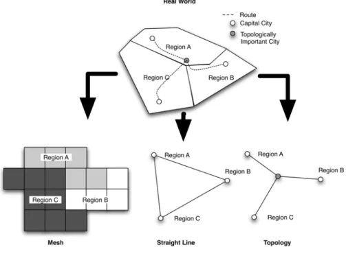
There are several ways to incorporate ‘geography’ into the NEG model (Figure 2). The first way is the ‘mesh’ or ‘grid’ representation, in which the region consists of many meshes or grids. Each mesh is treated as a place of production and consumption, connected to four or eight neighboring meshes. The second way is a ‘straight line’ representation, which simply connects cities, as places of production and consumption, with each other using straight lines; there is no topology, and geography means the distances between cities. The third way, adopted by the IDE-GSM, is to incorporate geography as ‘topology’ of cities3 and routes.
The ‘topology’ representation of geography has two major advantages over the mesh representation. Firstly, it makes it possible to incorporate a realistic choice of routes in logistics; the mesh representation does not necessarily incorporate ‘routes’ explicitly. A problem in topological representation is to calculate the minimal distance between any two cities considering every possible route between them. Fortunately, the Warshall-Floyd method provides a solution for this problem, and it is used in the IDE-GSM.
3
The variable ‘city’ used in the GSM refers to an administrative city. However, the GSM does not exclude the possibility of defining ‘city’ as a more realistic area according to actual economic activities.
137
Figure 2: Representations of Geography in the NEG model
It is also possible to add an ‘interchange city,’ having no population or industry, just to capture the realistic topology of cities and routes. It is also possible to put ‘border costs’ explicitly on routes crossing the border, enabling the model to take into account various costs at border controls. Furthermore, incorporating ‘routes’ explicitly makes it possible to incorporate differences in the quality of roads by setting different ‘average speeds’ for travelling on them. This is very useful when evaluating the effects of transport infrastructure development projects (see Figure 3).
The second advantage of the ‘topology’ representation of geography is that it requires less data concerning cities or points; the mesh representation requires various data for a large number of meshes. The first-generation IDE-GSM uses 361 capital cities and 184 topologically important cities to represent the whole of CSEA (continental Southeast Asia) (Figure 4). For instance, if the mesh representation is used in a 10 km by 10 km area, data would be required for more than 33,700 meshes for the region. Although a larger mesh may be used to reduce the number of meshes (100 km by 100 km with 337 meshes for example), this would be too vague to capture the geographical features of CSEA.
138
Figure 3: Gains in Regional GDP: East-West Economic Corridor vs. Baseline
Source: IDE-GSM estimation.
Note: For details of the simulation, see Appendix A.
Figure 4: Topology Representation of CSEA Countries
139
Compared with the ‘straight line’ representation, the ‘topology’ representation possesses a strong advantage, namely, its ability to incorporate routes between cities explicitly, while the data requirement other than route data is almost the same.
4. Nominal Compatibility with Realistic Statistics
4.1 Replicating the Reality
Productivity
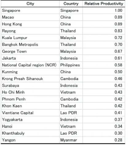
Whether using a standardized number (for instance, we set the nominal wage in Singapore equal to 1.0) or the actual number, a realistic simulation, when applied to policy analyses, needs to replicate the various statistics that are compatible with the actual data. We try to replicate the actual spatial structure of economic activities in a region, by constructing a proper model and calibrating key parameters, but it is not possible to fit the model-generated numbers to the real data perfectly. It is unavoidable that there remain ‘residuals.’ How can we handle these residuals? The easiest way is to assume that the levels of economic activity unexplained by the NEG model are the differences in ‘technology’ between regions. In our preliminary estimation, the relative manufacturing labour productivity of major cities in the CSEA region is shown in Table 1.
"%!
Table 1: Relative Productivity of Manufacturing Labour in CSEA (2005)
Source: Estimation by IDE-GSM.
Price indices
In NEG models, price indices play very important roles. For instance, the inter-regional labour mobility is determined by the differences in the real wage, which is calculated from the nominal wage and price indices. Although it is often difficult to obtain actual price indices by country or at the sub-national level, we need to check the validity of price indices by region and by industry. If the price indices are improper, we need to re-examine the data and reconsider the parameters.
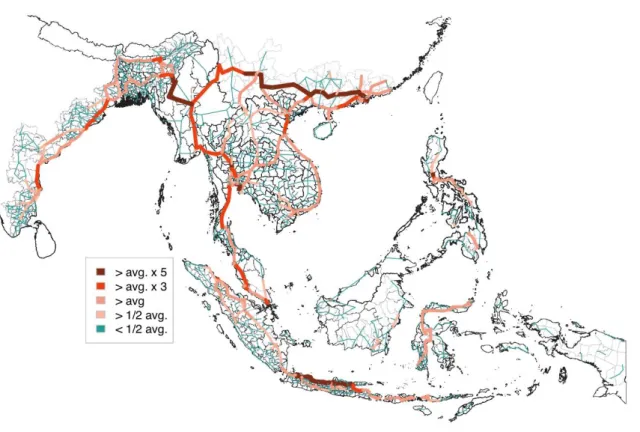
Traffic volume
In the IDE-GSM model, it is possible to calculate the traffic volume for every section of the routes. Figure 5 is an example of the relative land traffic volume by route. If the traffic volumes of some sections are unrealistically high or low, we need to reconsider the route data and the parameters in model choice decision. When calculating the traffic
141
volume, the IDE-GSM uses the value of the goods after subtracting the portion that is assumed to ‘melt’ during transport, meaning that the value of the goods is discounted by transport costs en route.
Figure 5: Estimated Relative Land Traffic Volume (2005)
Source: Estimated by IDE-GSM.
The Meaning of Steady State
The meaning of equilibrium or ‘steady state’ is different in theoretical analyses and realistic simulations. Equilibrium in the short term is essential for both theoretical analysis and realistic simulations, meaning that all variables need to be set to satisfy all the equations in the model, given the geographic distribution of population and economic activities.
On the other hand, equilibrium in long term carries a different importance for theoretical analyses and realistic simulations. In theoretical analyses, the speed of convergence to the ‘steady state’ is not a matter of concern. In realistic simulations, the speed of convergence matters a great deal in order to derive policy implications. For instance, assume that the simulation predicts a balanced distribution of economic
142
activity between currently high-income urban areas and low-income rural areas in the future. If this will happen in 10 to 20 years or so, we need no policy measure to facilitate balanced growth between urban areas and rural areas. On the other hand, if this will happen in 100 or more years, we cannot wait for the invisible hand to narrow the income gap between urban and rural areas.
Long-term equilibrium is very important in the analysis of the behaviors of the model. On the other hand, equilibrium might never be reached in a 20-year simulation by the IDE-GSM given the current speed of convergence; moreover, the long-term behavior of the model is not as critical for East Asia as it is for the EU case. One of the reasons for this is that international and intra-national wage differences in East Asia are so large compared with the EU that the answer to the concentrate-or-disperse question is not as sensitive to the parameters as in the EU, i.e., the agglomeration forces are generally stronger than dispersion forces, in East Asia, for the foreseeable future.
4.2 Setting the Parameters
In order to run the simulation properly, we need to identify various parameters properly. In the typical NEG simulation, some of the most important parameters are as follow.
a) Transport costs (T)
b) Elasticity of substitution ( ) c) Share of labour input ( ) d) Share in consumption ( )
The share of labour input and share in consumption are determined relatively easily from the I-O table, if available. On the other hand, transport costs and elasticity of substitution are difficult to obtain directly, meaning that we need to estimate them or apply the typical numbers presented by other studies.
In addition to these parameters, we need to determine the parameters for the ‘speed’ of adjustment. Specifically, we need to set the upper limits of inter-country, intra-country and inter-industry labour mobility separately. These parameters might be determined by an estimation based on the past data. In the current setting of the
143
IDE-GSM, international labour mobility is prohibited, and the inter-sectoral labour mobility is faster than inter-regional labour mobility within a country.
5. Growth and Distribution
How to incorporate economic growth in the NEG model is one of the important topics in constructing a realistic simulation model. There is the so-called NEGG (New Economic Geography and Growth) model, presented, for example, by Baldwin and Forslid (2000). The authors incorporated the (knowledge) capital production sector in the typical CP model and found that the periphery is relatively worse off by agglomeration, although it benefits from the overall growth of the economy in some cases. However, the NEGG model is an analytical model, and it is not easily applied to a realistic simulation.
Without incorporating a ‘growth engine’ sector in the model, there are three sources of endogenous growth in the IDE-GSM model, assuming the technology is different in each region and fixed thought the simulation period. Firstly, migration from a rural area, where the level of technology is generally low, to an urban area, where the level of technology is generally high, causes an increase in output in the urban area which exceeds the decrease in output in the rural area. Secondly, the job change within a region, from an industry in which the level of technology is generally low, to another industry in which the level of technology is generally high, causes an increase in output in the region. These two sources of growth are naturally extracted by the population dynamics, from a lower wage region/industry to a higher wage region/industry. Lastly, the external rate of population growth is given according to the predicted rate of population growth by UNESCAP, contributing to the endogenous economic growth. In addition to these ‘sustaining’ growth sources, there is ‘one-time’ growth when transport costs between cities are reduced by hypothetical infrastructure development.
It is a plausible idea to suggest the external rate of technological progress as another source of economic growth. However, when each region increases its productivity, it leads to the economic growth that exceeds the intended level because of the interaction of the increased productivity. Thus, it is difficult to set a ‘proper’ rate of
"%%
technological progress exogenously. It is also not easy to incorporate an ‘innovation’ sector that produces the knowledge capital which hikes the productivity of the region.
6. Specifying Industrial Sub-sectors
In the original CP model, there are two sectors, namely, agriculture and manufacturing. To make the model more realistic, we decided to divide the sectors into more sub-sectors. To make it possible for the IDE-GSM to derive more concrete policy implications, the industrial sectors in the current generation model are extended from three to seven. This extension enables the model to predict the impact of infrastructure development on each industry more precisely and to derive policy implications that are more industry-specific (see Figure 6).
Figure 6: Gains in GDP by the East-West Economic Corridor (10 years after)
Source: IDE-GSM estimation.
145
The first generation of the IDE-GSM has three sectors: (1) Agriculture, (2) manufacturing and (3) service. The service sector is incorporated simply as a sector that incurs extremely high transport costs, all other things being equal to the manufacturing sector. On the other hand, the second generation of the IDE-GSM has seven sectors, namely, (1) agriculture, (2a) automotive, (2b) electric and electronics, (2c) textile and garment, (2d) food processing, (2e) other manufacturing and (3) service. The third generation model maintains this sub-division of industry.
The basic structure of the model is unchanged from the first generation of the IDE-GSM, which is essentially based on the model introduced in Chapter 14 of Fujita, Krugman, and Venables (1999). Each sub-sector uses its own product and labour as inputs. This means that the input-output table in this world is filled with zeros except for the diagonal elements. This seems to be a radical simplification, but not too unrealistic given that the five sub-sectors are sufficiently differentiated from each other.
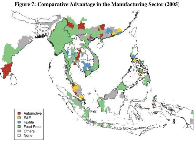
The principal problem in dividing the manufacturing sector is how to differentiate the several sub-sectors in the model. In addition to the initial geographical distribution of each sector (see Figure 7), there are four important parameters, or possible sources of difference, in this model, as mentioned in 4.2.
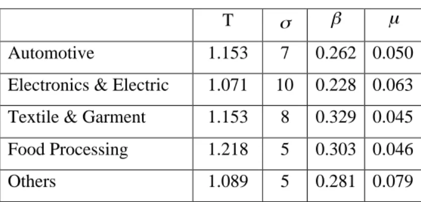
From various sources, we specify the parameters for each sector temporarily as shown in Table 2, and we assume these figures to be common to all countries.
Table 2: Parameters Specifying Each Industry T
Automotive 1.153 7 0.262 0.050 Electronics & Electric 1.071 10 0.228 0.063 Textile & Garment 1.153 8 0.329 0.045 Food Processing 1.218 5 0.303 0.046 Others 1.089 5 0.281 0.079
To make the model more realistic, the input-output table might be set to replicate reality more precisely. For instance, the automotive sector requires some input from the electronics sector. However, this direction of extension of the model raises two issues. Firstly, we need more data to construct a realistic input-output table, and ideally, it
146
should be different by region. For East Asia, it is quite difficult to construct a reliable IO table for some countries at this moment, and constructing an IO-table by sub-national region is a challenge. Secondly, we need to distinguish finished products and intermediate products explicitly in this kind of realistic IO structure. However, it is also difficult to set the proper parameters for the goods to reflect whether they are finished or intermediate goods.
Figure 7: Comparative Advantage in the Manufacturing Sector (2005)
Source: KGIK dataset used for the IDE-GSM. Note: For details of the figure, see Appendix B.
Another important issue in dividing the sectors is how to handle the service sector. In the IDE-GSM, the service sector is treated as a sector that 1) incurs large transport costs and 2) offers highly differentiated goods, i.e., has low . However, the degree of differentiation in the service sector is arguable. If we assume the sector is like ‘barbers’, the degree of the differentiation should be low, and the transport costs should be high. On the other hand, if we assume the sector is like ‘tourism,’ then the degree of
147
differentiation should be high, and the transport costs should be relatively low. It is not an easy task to properly set and T for the service sector as a whole.
7. Problems in Incorporating Transport Costs
7.1 Level of Transport Costs
Most of the NEG models, including the CP model, incorporate transport costs in a special form, namely, as ‘iceberg’ transport costs. The beauty of this setting is that we do not need to incorporate the logistic industry explicitly, thereby keeping the model simple. The form of the transport cost function can be linear or exponential to the distance.
The largest problem in incorporating transport costs into a simulation model is how to set the level of transport costs properly. Recently, there have appeared various empirical studies on transport costs. For instance, Hummels (1999) estimated the elasticity of substitution and the average freight costs and by sector. Anderson and Wincoop (2004) assert that the tax equivalent of more broadly defined transaction costs in a developed country is 170%. However, there is no consensus on the ‘proper’ level of transport costs to be used in NEG-based simulations so far.
To make matters worse, we need to set different levels of transport costs for different industries. The components of transport costs, or ‘transaction costs’ generally, are quite different for each industry. For one industry, transport costs are basically the payment to the logistic service. On the other hand, another industry may regard the time to delivery as an important component of transport costs. How to set the function of transport costs for each industry is a formidable problem in the construction of realistic simulation models.
The first two generations of the IDE-GSM implemented the traditional ‘iceberg’ transport costs, and transport costs are defined by industry. Thus, for instance,
T=1.153 means that 1.00 out of 1.153 units of goods shipped from one part of
continental Southeast Asia (CSEA) arrived in another part of CSEA. From this, it can be understood that bringing goods from one part of CSEA to another requires a 15.3%
148 overhead cost on the price of the goods.
In the third-generation IDE-GSM model, transport costs are handled in a completely different way from that of the past two models. Firstly, we calculate the money-equivalent transport costs of transporting one 20-foot container by industry, mode and distance. Then, we calculate the percentage of theses transport costs against the value of one 20-foot container filled with each good. This number is treated as , the transport costs between cities i and j for goods k by mode m.
7.2 Modal Choice
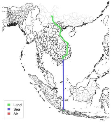
Related to the problem mentioned in the previous sub-section, the modal choice of road, sea or air transport is another important issue. Basically, we need to consider both the money costs of transportation and the time costs of transportation, bearing in mind the optimum modal choice by industrial sector. Some industries may take the time costs seriously, choosing the faster mode of transportation although the money costs are higher, or vice versa. Figures 8-1 through 8-3 are the sample models of the modal choices that consider both money costs and time costs by mode and by industry. For testing purposes, only one air route is included, and that is between Singapore and Jakarta. It is quite interesting to observe that the modal choice differs as the time costs differ.
149
Figure 8-1: Route from Jakarta to Kunming (low time costs)
150
Figure 8-3: Route from Jakarta to Kunming (high time costs)
8. LACK OF DATA
The highest bar in the development of a realistic NEG model in East Asia is not in the modeling but in the lack of a reliable geo-economic dataset. Firstly, more precise regional economic and demographic data is needed at the sub-national level in each country and at the sub-provincial level in China and India. Specifically, the establishment of uniform territorial units for geographical statistics in East Asia is crucial. Without such uniform territorial units, various statistics cannot be compared directly across countries. For example, it is not proper to compare the concentration of populations at the ‘state’ level in Malaysia versus those at the ‘provincial’ level in China. In Europe, EUROSTAT established the Nomenclature of Territorial Units for Statistics (NUTS) more than 25 years ago. NUTS enables geographical analysis and formation of regional policies based on a single uniform breakdown of territorial units for regional statistics. An East Asian counterpart of NUTS (perhaps called EA-NUTS) seems necessary as well. With EA-NUTS, basic social and economic information such as population, GDP, industrial structure, and employment by sector for each sub-region
151
could be collected or recompiled from existing datasets obtained from statistical departments of member countries.
Secondly, more precise data on routes and infrastructure connecting regions is needed. Information on the main routes between regions such as physical distance, time distance, topology, and mode of transport (road, railway, sea, and air) appears indispensable. Data on ‘border costs’ such as tariffs and time-costs due to inefficient customs clearance seems crucial. It may be necessary to measure and continuously update information on routes and border costs by conducting experimental distributions of goods and actual drives.
9. CONCLUSION
In this chapter, the author examined the various difficulties in developing a realistic simulation based on NEG, especially for East Asia, and presented some ways to resolve the difficulties in certain cases. At this point in time, there exists an obvious insufficiency of accurate economic data at the sub-national level in East Asia. To cope with this, the IDE-GSM selected ‘topology representation’ of geography as a solution.
However, the construction of a unified geographical dataset for East Asia as swiftly as possible is indispensable. Without such a dataset, researchers will continue to experience serious difficulties in checking the validity of models by comparing past and current data. Among other drawbacks, we will also be unable to gain data on the historical transitions in the geographical distribution of economic activity in East Asia, which is expected to be a valuable test bed for various studies on economic geography.
In addition to data problems, there are various issues to be addressed in model building, such as estimating and setting the parameters properly, handling economic growth in the model, replicating diverse industries in a manner that captures the differences and incorporating a realistic modal choice in the model. The task of resolving these issues in a tractable framework of numerical simulation models is an intricate challenge.
The more realistic the model becomes, the more we need to identify additional parameters and check the reality of an increasing number of variables. It is
152
not possible to replicate reality perfectly while maintaining the legitimacy of the model from the viewpoint of the theory of new economic geography. Thus, it is important to specify what aspects of the economy we need to simulate and then to construct the model accordingly.
References
Anderson, E. James and Eric van Wincoop. 2004. Trade Costs. Journal of Economic
Literature. Vol XLII, pp.691-751.
Baldwin, E. Richard and Rikard Forslid. 2000. The Core-Periphery Model and Endogenous Growth: Stabilizing and Destablizing Integration. Economica. Vol. 67, pp.307-324.
Bosker, M., Brakman, S., Garretsen, H., and M. Schramm. 2007. Adding Geography to The New Economic Geography. CESifo Working Paker No. 2038.
Bröcker, J., Capello, R., Lundqvist, L.Meyer, R., Rouwendal, J., Schneekloth, N., Spairani,A., Spangenberg, M., Spiekermann, K. and Wegener, M. 2004. Territorial Impact of EU Transport and TEN Policies:Final Report of Action 2.1.1 of the European Spatial Planning Observation Network ESPON 2006, Institut für Regionalforschung, Christian-Albrechts-Universität Kiel.
Fingleton, Bernard. 2006. The new economic geography versus urban economics: an evaluation using local wage rates in Great Britain. Oxford Economic Papers 58. Pp.501-530.
Fujita, Masahisa. Paul Krugman. and Anthony J. Venables. 1999. The Spatial Economy: Cities, Regions, and International Trade. Cambridge, MA: MIT Press. Fujita, Masahisa and Tomoya Mori. 2005. Frontiers of New Economic Geography.
Papers in Regional Science, Vol.84 No.3. pp. 377-405.
Hummels, David. 1999. Toward a Geography of Trade Costs. Working Paper. Purdue University.
Krugman, Paul. 1991. Increasing Returns and Economic Geography. Journal of
Political Economy. Vol. 99, pp. 483-499.
153 Vol.37. pp293-298
Kumagai, Satoru, Toshitaka Gokan, Isono Ikumo and Souknilanh Keola. 2008. The IDE Geographical Simulation Model: Predicting Long-Term Effects of Infrastructure Development Projects, IDE Discussion Papar 159.
Puga, Diego. 1999. The rise and fall of regional inequality. European Economic Review Vol. 43, pp.303-334.
Stelder, Dirk. 2005. Where Do Cities Form? A Geographical Agglomeration Model for Europe. Journal of Regional Science. Vol. 45. No.4, pp. 657-679.
Teixeira, Antonio Carlos. 2006. Transport policies in light of the new economic geography: The Portuguese experience, Regional Science and Urban Economics, Vol. 36, pp.450-466.
154
APPENDIX A
In the simulation, several macroeconomic and demographic parameters may be held constant, and only logistic settings (by scenario) changed. The following macro parameters are then maintained across scenarios:
• The national population of each country is assumed to increase at the rate forecasted by the United Nations Population Fund (UNFPA) until the year 2025;
• There is no immigration between CSEA and the rest of the world.
The assumptions in the baseline scenario are as follow:
• An Asian highway networks exist, and cars can travel at 30km/h on it. • Border costs, or times required for customs clearance, are as follow:
Singapore – Malaysia 2.0 hours Malaysia – Thailand 8.0 hours All Other National Borders 24.0 hours
The assumptions in the EWEC scenario are as follows:
• Cars can travel on the EWEC at 60 km/h after the year 2011 and on other Asian highways at 30km/h.
• Border controls along the EWEC are as efficient as those at the Singapore-Malaysia border (taking 2.0 hours to cross national borders) after the year 2011.
The gains in GDP are calculated by comparing the EWEC scenario against the baseline scenario in the year 2020.
155
APPENDIX B
GDP per capita by sub-national region in this study is constructed from various sources, and mainly from the national statistical office in each country, by the Kumagai-Gokan-Isono-Keola (hereinafter, ‘KGIK dataset’). Figure 7 presents the sector that has highest Revealed Comparative Advantage-like (RCA) index among five manufacturing sectors by region. A region with a manufacturing sector amounting to less than 5% of its total GDP is categorised as having ‘none.’