Numerical analysis of Io's atmosphere based on a model Boltzmann equation : Unsteady behavior during eclipse (Mathematical Analysis in Fluid and Gas Dynamics)

Numerical

analysis

of Io’s

atmosphere

based

on

a model

Boltzmann equation: Unsteady behavior

during eclipse

Shingo

Kosuge

Department

of Mechanical Engineering and Science, Kyoto University

1

Introduction

$Io$ is a satellite of Jupiter. The observations made by NASA’s spacecrafts in the $1970s$

(Pioneer and Voyager probes) revealed the existence of volcanic activities and

a

thin atmosphere mainly composed of sulfur dioxide $(SO_{2})$ gas. The surface temperature of Io

is considered to vary according to the sunlight between about

90

$K$ and

130

$K$ (except

near

volcanos). The phase transition of $SO_{2}$

occurs

in this temperature

range:

the $SO_{2}$

gas condenses to form $a$ (very thin) layer of frost

on

the ground during the night and,

as

a result, the atmosphere may almost vanish; conversely, the frost sublimates and the atmosphere is restored during the daytime. The dynamics of $Io$’s atmosphere under

sublimation and condensation of$SO_{2}$ has been studied for a longtime (see, e.g., Refs. [1,

2, 3, 4] and references therein).

The above-mentioned process of atmospheric collapse and reformation is expected to take place also during and after eclipse, during which Io is in the shadow of Jupiter. Moore et. al. [5] tackled such a problem for thefirst time: they carried out a numerical analysisof the Boltzmann equation by the direct simulation Monte Carlo (DSMC) method [6, 7] to investigate the unsteady one-dimensional behavior of the atmosphere in eclipse. In Ref. [5], the atmosphere

was

treated

as

a binary mixture of $SO_{2}$ and another minor

component ($SO$

or

$O_{2}$), the latter of which is (partially) noncondensable. The results

in Ref. [5] reveal the effect of the noncondensable gas:

a

trace of noncondensable gas

carried by the condensing flow of $SO_{2}$ accumulates on the surface at the early stage of

eclipse and then acts

as a

barrier to furthercondensation to delay the atmospheric collapse significantly. In the meantime, little information

on

the time evolution and structure of the flow field is available from Ref. [5], mainly because of the stochastic noise inherent in the DSMC results.

In this report, we introduce

our

recent results in Refs. [8, 9], where essentially the

same

problem

as

in Ref. [5]

was

studied through

a

different approach after making

some

simplifications. First we adopted the model Boltzmann equation proposed in Ref. [10], instead of the full Boltzmann equation, forcomputationalconvenience. Secondwe focused on the effect of the noncondensable gas only, because it was expected to be dominant;

we

omitted all other effects taken into account in the previous DSMC analysis [5], such

as

the

effect

of plasma impingement

from

the outer space, that of molecular internal structure, and

so on.

Then

we

could perform an accurate deterministic computation by

means

ofa finite-difference method at a reasonablecomputational cost. In spite of those simplifications, however, the overall behavior (the column density of $SO_{2}$) during eclipse

obtainedin

our

study is quite similar to the previous result [5]. Moreover,

as

will be seen later in Sec. 5, our solutions with higher temporal and spatial resolution reveal

some new

phenomena (waves in the profiles of macroscopic quantities and

an

oscillatory motion), which

were

not explored in Ref. [5].

2

Problem and assumptions

Consider an atmospheric column

over

a fixed point

on

Io’s surface

near

the equator belonging to thesub-Jovian

hemisphere.1

The groundis located at $X_{1}=0$ and is covered

by the frost of$SO_{2}$, where _{$X[=(X_{1}, X_{2}, X_{3})]$} be the spacerectangular

coordinates.2

The

atmosphere extends

over

the half-space$X_{1}>0$and iscomposed of$SO_{2}$ vaporand another

noncondensable gas, $SO$ or $O_{2}^{3}$ The eclipse starts at time _$t=0$ and lasts until _$t=120$

$\min$. The initial atmosphere is assumed to be in _{a saturated equilibrium state at rest}

with uniform temperature $T_{0}$. The surface temperature _{$T_{w}$}, which coincides with $T_{0}$ at

$t=0$, varies with time_{according to the change of insolation [see Eq. (11) below] and then} condensation or sublimation of$SO_{2}$ may

occur.

We investigate unsteady behavior of the

atmospheric column during eclipse under the following assumptions: (i) the behavior of the atmosphere is

described

by the model Boltzmann equation for mixtures proposed in Ref. [10]; (ii) the vapor ($SO_{2}$ gas) obeys the complete-condensation boundary condition

on

the surface [see Eq. (7) below]; (iii) the noncondensable gas ($SO$

or

$O_{2}$) obeys the

diffuse-reflection boundary condition on the surface; (iv) the surface and the atmosphere

are horizontally uniform [in thelength scale ofthe pressure scaleheight $H$ $(\sim 7-9 km)$ _of

the atmosphere], sothat the problem

can

be treated as aspatially 1-$D$problem depending

on $X_{1}$ only.

$\overline{1As}$

aresult of tidal locking, Io always shows thesameside(thesub-Jovianhemisphere) to Jupiter,sothat the eclipse

does not much effect the anti-Jovian hemisphere.

2Thecurvature of thesurface isignorableinthepresentproblem.

3

Formulation

Inthe following, the vapor ($SO_{2}$ gas) and noncondensablegas ($SO$or$O_{2}$) willbe referred

to

as

species $A$ and $B$, respectively. The Greek letters $\alpha$ and $\beta$ will be used to represent

the species, i.e., $\alpha,$$\beta=\{A, B\}.$

Let

us

denote the velocity distribution function (VDF)

of molecules

of species $\alpha$

as

$F^{\alpha}=F^{\alpha}(t, X_{1}, \xi)$, where $\xi[=(\xi_{1}, \xi_{2}, \xi_{3})]$ is the molecular velocity. The macroscopic

quantities, such

as

the number density $n^{\alpha}$, flow velocity $v^{\alpha}[=(v_{1}^{\alpha}, v_{2}^{\alpha}, v_{3}^{\alpha})]$, pressure $p^{\alpha},$

and temperature $T^{\alpha}$ of species $\alpha$,

are

defined

as

the moments of $F^{\alpha}$

as

follows:

$n^{\alpha}= \int F^{\alpha}d\xi, v^{\alpha}=\frac{1}{n^{\alpha}}\int\xi F^{\alpha}d\xi,$

(1)

$p^{\alpha}=kn^{\alpha}T^{\alpha}= \frac{1}{3}\int m^{\alpha}|\xi-v^{\alpha}|^{2}F^{\alpha}d\xi,$

where $m^{\alpha}$ is the molecular

mass

of species

$\alpha,$ $k$ is the Boltzmann constant, and $d\xi=$

$d\xi_{1}d\xi_{2}d\xi_{3}$. The domain of integration is the whole space of$\xi$. The corresponding

quanti-ties of the totalmixture, i.e., the number density$n$, flow velocity$v[=(v_{1}, v_{2}, v_{3})]$,

pressure

$p$, and temperature $T$ of the mixture,

are

given by

$n= \sum_{\alpha=A,B}n^{\alpha}, v=\sum_{\alpha=A,B}m^{\alpha}n^{\alpha}v^{\alpha}/\sum_{\alpha=A,B}m^{\alpha}n^{\alpha},$

(2)

$p=knT= \sum_{\alpha=A,B}(p^{\alpha}+\frac{1}{3}m^{\alpha}n^{\alpha}|v^{\alpha}-v|^{2})$ .

Note that the horizontal components of the flow velocity will be ignored (i.e., $v_{2}^{\alpha}=v_{3}^{\alpha}=$ $v_{2}=v_{3}=0)$ in the actual analysis, whereas they are left in the formulation.

3.1 Model Boltzmann equation

The model Boltzmann equation in Ref. [10] for the present problem may be written

as

follows:

$\frac{\partial F^{\alpha}}{\partial t}+\xi_{1}\frac{\partial F^{\alpha}}{\partial X_{1}}-g\frac{\partial F^{\alpha}}{\partial\xi_{1}}=K^{\alpha}(M^{\alpha}-F^{\alpha}) , (\alpha=A, B)$. (3)

Here, $g(=1.8m/s^{2})$ _{is the gravitational acceleration}

on

Io, which is treated

as a

constant

since the scale height $H$ is much smaller than Io’s radius $R$ $(=1820 km)$. For the

same

reason, the effect of planetaryrotation (theCoriolis and centrifugal force) is omitted. The

$K^{\alpha}$ and $M^{\alpha}$

are

defined by

$K^{\alpha}= \sum_{\beta=A,B}K^{\beta\alpha}n^{\beta},$

(4)

The $K^{\beta\alpha}(=K^{\alpha\beta})$ is

a

positive constant, that determines the collision frequency of

an

$\alpha$-species molecule with $\beta$-species molecules via$K^{\beta\alpha}n^{\beta}$. Thus, the above $K^{\alpha}$ corresponds

to the total collision frequency of

an

$\alpha$ molecule. The velocity $v^{(\alpha)}$ and temperature $T^{(\alpha)}$

ofthe Maxwellian $M^{\alpha}$

are

defined by

$v^{(\alpha)}=v^{\alpha}+ \frac{2}{m^{\alpha}K^{\alpha}}\sum_{\beta=A,B}\mu^{\beta\alpha}\Omega^{\beta\alpha}n^{\beta}(v^{\beta}-v^{\alpha})$, (5a)

$T^{(\alpha)}=T^{\alpha}- \frac{m^{\alpha}}{3k}|v^{(\alpha)}-v^{\alpha}|^{2}$

$+ \frac{4}{K^{\alpha}}\sum_{\beta=A,B}\frac{\mu^{\beta\alpha}\Omega^{\beta\alpha}n^{\beta}}{m^{\beta}+m^{\alpha}}(T^{\beta}-T^{\alpha}+\frac{m^{\beta}}{3k}|v^{\beta}-v^{\alpha}|^{2})$ , (5b)

where $\mu^{\beta\alpha}[=m^{\beta}m^{\alpha}/(m^{\beta}+m^{\alpha})]$ is the reduced

mass

and $\Omega^{\beta\alpha}(=\Omega^{\alpha\beta})$ is

an

additional

positive constant; the positivity of $T^{(\alpha)}$ follows if $\Omega^{\beta\alpha}\leq K^{\beta\alpha}$. Note that Eq. (1) is

necessary to complete the model equation because$n^{\alpha},$ $v^{\alpha}$, and $T^{\alpha}$ appearin Eqs. (4) and

(5).

This model

was

designed in such a way that, by adjusting $\Omega^{\beta\alpha}$

, the momentum and energyexchanges betweendifferent speciescanbe the same as thosefor (pseudo-)Maxwell molecules with an arbitrary value of the angular cutoff parameter (see, e.g., Ref. [11]). In the present study, however, this property is not used for specifying thevalue of $\Omega^{\beta\alpha}$. We

first specify $K^{AA}$ by the _relation

$K^{AA}=4d^{2}(\pi kT_{0}/m^{A})^{1/2}$, (6)

where $d(=7.16\cross 10^{-10}m)$ is the nominal diameter of an $SO_{2}$ molecule. This

rela-tion means that the molecular

mean

free path with respect to $SO_{2}-SO_{2}$ collisions in an

equilibrium state with temperature $T_{0}$ for the model equation is equal to that for the

hard-sphere gas with molecular diameter $d$. Then, for simplicity, $K^{BB},$ $K^{BA}$, and $\Omega^{BA}$

are

all assumed to be identical with $K^{AA}$ [note that $\Omega^{AA}$ and $\Omega^{BB}$ are unnecessary; see

Eq. (5)$]$. Therefore, pseudo-Maxwell behavior of the molecules is not enforced in the present study.

3.2 Initial and boundary conditions

The boundary condition on the surface is written as follows. For $X_{1}=0$ and $\xi_{1}>0,$

$F^{\alpha}=n_{w}^{\alpha}( \frac{m^{\alpha}}{2\pi kT_{w}})^{3/2}\exp(-\frac{m^{\alpha}|\xi|^{2}}{2kT_{w}})$ , (7a)

Here

$p_{w}^{A}$ is the

saturated vapor pressure of

$SO_{2}$ at temperature $T_{w}$ and is

given

by the

Clausius-Clapeyron relation:

$p_{w}^{A}=\Pi\exp(-\Gamma/T_{w})$,

(8)

$(\Pi=1.516\cross 10^{13}$ Pa and $\Gamma=4510K)$.

In the present problem, thevariation of$T_{w}$ and corresponding$p_{w}^{A}$ withtimewould induce

the unsteady motion ofthe atmosphere through the boundary condition (7). The initial condition is written

as

follows. At $t=0,$

$F^{\alpha}=n_{0}^{\alpha}( \frac{m^{\alpha}}{2\pi kT_{0}})^{3/2}\exp(-\frac{m^{\alpha}(|\xi|^{2}+2gX_{1})}{2kT_{0}})$. (9)

Here $n_{0}^{\alpha}$ is the initial number density ofspecies $\alpha$ on the surface $(X_{1}=0);n_{0}^{A}=p_{0}^{A}/kT_{0}$

with $p_{0}^{A}$ being the saturated vapor pressure at temperature $T_{0}$ [i.e., $p_{0}^{A}$ is givenby Eq. (8)

with $T_{w}$ being replaced by $T_{0}$]. The initial temperature $T_{0}$ will be chosen in the next

section. Theconcentration $\chi^{B}$of the noncondensable gas in the initial atmospheric column

is written

as

$\chi^{B}=\int_{0}^{\infty}n^{B}(t=0)dX_{1}/\int_{0}^{\infty}n(t=0)dX_{1}$

(10)

$= \frac{(n_{0}^{B}/m^{B})}{(n_{0}^{A}/m^{A})+(n_{0}^{B}/m^{B})}.$

In the following, the amount of the noncondensable gas will be specified by $\chi^{B}$, instead

of$n_{0}^{B}.$

3.3 Surface temperature

The surface temperature $T_{w}$ is determined by the

same

differential equation

as

that in

Ref. [5]:

$\frac{dT_{w}}{dt}=\{\begin{array}{ll}A\sigma(T_{{\rm Min}}^{4}-T_{w}^{4}) , for 0\leq t\leq 120\min,A\sigma(T_{E}^{4}-T_{w}^{4}) , for t>120\min,\end{array}$ (11)

where $\sigma$ is the Stefan-Boltzmann constant and $A=\epsilon/C$ with $\epsilon$ being the bolometric emissivity and $C$ the heat capacity per unit

area

ofthe surface. The $T_{E}$ is

an

equilibrium

temperature defined as

$T_{E}=\{\begin{array}{ll}(T_{{\rm Max}}-T_{{\rm Min}})\cos^{1/4}\theta+T_{{\rm Min}}, for \theta\leq 90^{o},T_{{\rm Min}}, for \theta>90^{o},\end{array}$ (12)

where $\theta$ is the solar zenith angle (SZA), whichvaries with time according to the diurnal motion of the sun. The maximum and minimum of $T_{E}$ are fixed

as

$T_{{\rm Max}}=120K$ and

$\frac{}{}\frac{TABLE1:Simulationcases}{CaseT_{0}(K)Longitude(^{\circ})GasB(\chi^{B})A^{-1}(J/m^{2}K),111069-(0)350}$ 2 110 69 $SO$ (0.35) 350 3 110 69 $SO$ (0.35) 700 4 110 69 $SO$ (0.35) 175

$5 110 69 O_{2}(0.35) 350$

$6 110 69 O_{2}(0.07) 350$

$7 115 52 -(0) 350$

8 115 52 $SO$ (0.22) 350

$9 120 351 -(0) 350$

10 120 351 $SO$ (0.03) 350

The initial temperature $T_{0}$ appearing in Eq. (9) is chosen as $T_{0}=T_{E}(t=0)$ using

Eq. (12), after we specify the location of the atmospheric column (i.e., the longitude and latitude) and calculate the SZA $\theta$ as a function of time $t$ (note that $t=0$ is defined to

be the time when eclipse starts). It should be noted that the above $T_{w}$ is influenced only

by the insolation and not by the atmospheric behavior (i.e., not by the latent heat and sensible heat from the gas), since the former is dominant. We solve Eq. (11) with the

initial condition $T_{w}(t=0)=T_{0}$ to obtain $T_{w}(t)$ beforehand.

4

Numerical analysis

We first eliminate the molecular-velocity variables $\xi_{2}$ and $\xi_{3}$ from the initial-boundary

value problem (3), (7), and (9) by introducing appropriate marginal VDF’s. Then, the reduced problem with three independent variables $t,$ $X_{1}$, and $\xi_{1}$ is solved by a

finite-difference method. We used (i) animplicit scheme in Ref. [12] where the derivatives with respect to $X_{1}$ and $\xi_{1}$

are

expressed by a $2nd$-order up-wind finite-difference (see, e.g.,

Ref. [13]$)$ and (ii) $2nd$-order Runge-Kutta (Heun’s) scheme along the characteristics of

Eq. (3) in combination with the interpolation method devised in Ref. [14]. In the latter scheme, because of the properties of the method in Ref. [14], the transient waves tend to be more accurately captured without overshoots in the profiles of the macroscopic quan-tities (and in those of the VDF’s). However,

as

in the cubic interpolated pseudo-particle (CIP) method [15], equations for the derivatives of $F^{\alpha}$ must be solved simultaneously.

Thus the latter requires larger amount of computations (and involves

some

difficulty in the treatment of boundary conditions for the derivatives). To compensate the increased amount of computations, we performed a parallel computing (the latter is an explicit

$\vee\wedge$ $f_{\neg}^{*}$

$t$(lllin) $t( \min)$

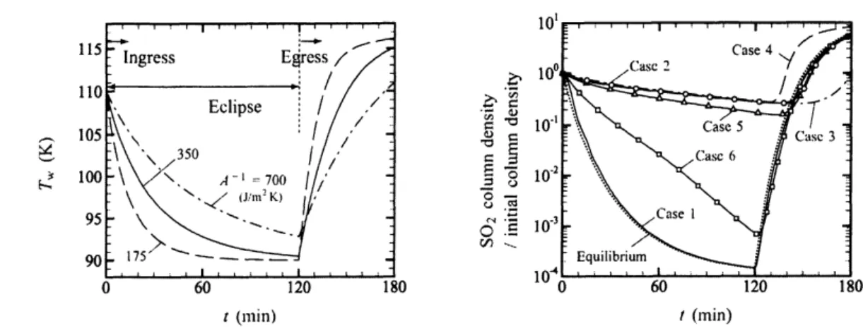
FIGURE 1: Surface Temperature $T_{w}$ and $SO_{2}$ column density vs. time in the case of _{$T_{0}=110$} $K.$

The initial $SO_{2}$ columndensity is $1.2386\cross 10^{20}\neq/m^{2}$. The dotted line in the right panelindicates the

theoretical value for pure $SO_{2}$ atmosphere in an isothermal saturated equilibrium state at rest when

$A^{-1}=350J/m^{2}K.$

scheme).

The results shown in the next section

were

obtained by scheme (ii), while the details of the method

are

omitted here [some test

runs

with scheme (i)

were

also performed and

gave

roughly the

same

results]. In the computation,

we

limit the range of$X_{1}$ up to $X_{1}\sim$

$282-313$ km and impose the specular-reflection condition at the upper $boundary^{4}$; the

minimum grid intervalsfor $T_{0}=110,115$, and 120 $K$ are, respectively, 15.9 _$m,$ $8.3m$, and

4.3 $m$ at $X_{1}=0$; the maximum intervals

are

about 0.3–1.1 km at the upper boundary.

The range

of

$\xi_{1}$ is limited

as

$|\xi_{1}|\leq 8c_{0}$, where $c_{0}[=(2kT_{0}/m^{A})^{1/2}]$ is about

173

$m/s$ for

$T_{0}=115K$; the minimum and maximum grid intervals

are 0.005

$c_{0}$ at $\xi_{1}=0$ and $0.045c_{0}$

at $\xi_{1}=\pm 8c_{0}$, respectively. The time steps

are

about 4.7 ms for $T_{0}=110$ and 115 $K$ and

2.3

ms

for 120 $K.$

5

Results

We consider Cases $1-10$ listed in Table 1; for simplicity, the column located in the

equator (orlatitude $0^{o}$) is considered in all the cases. The values of parameters in Table 1

were cited from Ref. [5].

Figure 1 shows the variations ofthe surface temperature and of the column density of

$SO_{2}$ in the

case

of $T_{0}=110$ K. The column density of pure $SO_{2}$ atmosphere (Case 1)

decreases significantly at the end ofeclipse, whereas in the

case

of mixtures the decrease

4Thiscondition wasusedto fixthetotal amountof thenoncondensable gasinthe column. $A$vacuumconditionforthe

(a)

$X_{1}$ (km) $X_{1}$ (km) $X_{1}$ (km)

(b)

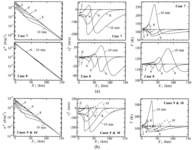
FIGURE 2: Profiles of the macroscopic quantities at every 2 minutes during the first 10 minutes after ingress. (a) Cases 7and 8, and (b) Cases 9 (solidhne) and 10 (dashed line). In (b), eachof thedashed lines approaches the corresponding solidline for thesame$t$ as $X_{1}arrow\infty.$

is hindered by the noncondensablegas [see Fig. 3(b) below]. The effects of the gasspecies

$(i.e., the$molecular$mass$ratio$m^{B}/m^{A})$, concentration$\chi^{B}$, and heat capacity of thesurface

$(\sim A^{-1})$

are

also examined. Except for

some

minor differences, the overall behavior of

the column shown in Fig. 1

seems

to be close to the corresponding result of the previous DSMC analysis (i.e., Fig. 8 in Ref. [5]).

5.1 During eclipse

Figure2showstheprofiles of macroscopic quantities at the beginning of eclipse. InCases 7 and 9 (pure$SO_{2}$), afast condensing flow is induced, and, as aresult, anexpansion

wave

(a)Case7 (b)Cabe8

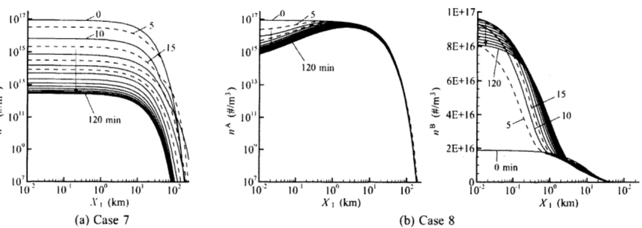
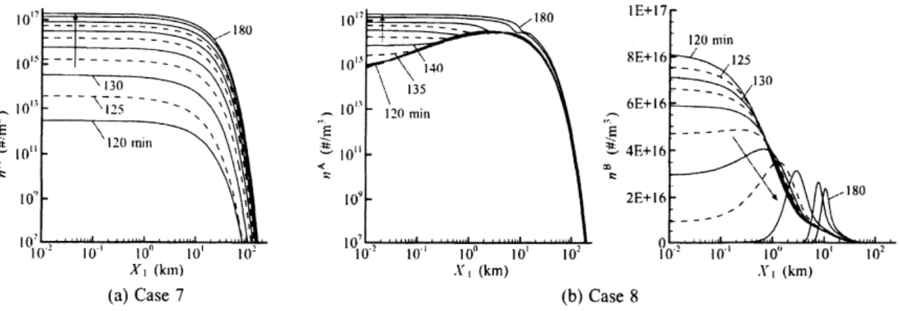
FIGURE 3: Number density profiles during eclipse. (a) Case 7and (b) Case 8. The solidline indicates

profiles at every 10 minutes $(t=0,10, \ldots, 120\min)$, _{and the dashed line those at $t=5,15,25$, and 35}

$\min$ in (a) and those at $t=5$ and 15 $\min$in (b).

the surface. While propagating upward, the shock

wave

stretches rapidly because the background pressure decays exponentially with altitude (thus the local

mean

free path grows exponentially). In Cases 8 and 10 (mixture), the condensing flow is relatively slow because of thehindrance by the noncondensable gas [see Fig. 3(b) below]. The expansion

wave

is sent

as

in the pure $SO_{2}$ case, but is immediately followed by a relatively weak

compression

wave.

Figure 3 shows the profiles of the number density in Cases 7 and 8 during eclipse. In

Case

7

(pure $SO_{2}$), the number density decreases at all altitudes until the end of eclipse

except at$t \sim 10-30\min$_. During that timeperiod, the number density _at high altitudes

$(X_{1}>\sim 100 km)$ is increased temporarily by the passage ofthe shock

wave

seen

inFig. 2.

In Case 8 (mixture), the number density of $SO_{2}$ decreases only in the neighborhood of

thesurface and hardly changes at high altitudes. This is because the noncondensablegas, which is carried by the condensing flow of$SO_{2}$to thesurfaceand accumulates there, forms

thepartialbarriertotheatmospheric collapse. Thenumberdensityof thenoncondensable gas

near

the surface increasesrapidly until$t \sim 20\min$and thenstartsto decrease because

of the upward selfdiffusion.

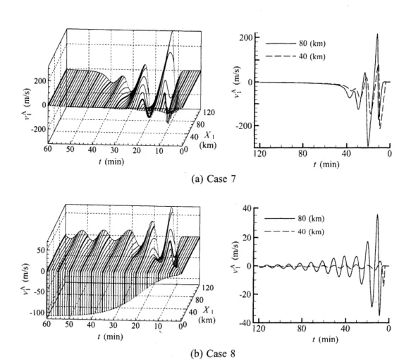
Figures 4 and 5 show, respectively, the profiles of the flow velocity and temperature in

Cases 7 and 8 during eclipse. The oscillatory behavior

seen

in the figures is produced by

waves

which,

as

those in Fig. 2, appear in the lower atmosphere and propagate upward successively. In Case 7, the amplitude of oscillation is large and thus

a

very fast flow and high temperature may appear instantaneously, especially at high altitudes. The oscillation decays rapidly with time and almost

ceases

until $t \sim 40\min$. In Case 8, while

$t( \min)$ 120 (a)Case 7 80 40 $0$ $t( \min)$ $t(r\iota\tau i\mathfrak{n})$ (b) Case8

FIGURE 4: Profiles of the flow velocity$v_{1}^{A}$ at every minute(left panel) and thecrosssectionsat$X_{1}\simeq 40$

and80 km (right panel). (a) Case 7 and (b) Case 8. The thick line in the left panelindicates profiles at every 5 minutes.

continuesuntil the end ofeclipseexcept nearthe surface. The oscillation period measured from the right panels of Figs. 4(b) and 5(b) is about 10 $\min$, whereas the Brunt-V\"ais\"al\"a

period for the initial isothermal atmosphere computed by a textbook formula is about

11.5 $\min$. In Case 8, a fast condensing flow in the close vicinity of the surface remains

until the end of eclipse. This is because the $SO_{2}$ density

on

the surface is kept much

higher than the saturation density by theeffect of the noncondensable gas [see Fig. $3(b)$].

The temperature in Case 8oscillates around the initial temperature $(T_{0}=115K)$ in most

parts ofthe atmosphere. The atmosphere is cooled only

near

the surface via conduction. 5.2 After egress

Figure 6 shows the profiles of the number density in Cases 7 and 8 afteregress. In Case 7, the number density starts to increase immediately after egress and the initial density

$\hat{i4\vee}$ $k$

$120 80 40 0$

$t( \min)$ $t( \min)$ (a)Case 7

$120 80 40 0$

$t( \min)$ _{$\prime(\min)$} (b) Case8

FIGURE 5: Profiles of the temperature$T$ateveryminute (left panel) andthecrosssections at $X_{1}\simeq 40$

and 80 km (right panel). (a) Case 7 and (b) Case 8. The thick linein theleft panel indicates profiles at

every 5 minutes.

(a) Case 7 (b) Case8

FIGURE 6: Number density profiles after egress. (a) Case 7 and (b) Case 8. The solid line indicates

profiles at every 10 minutes $(t=120,130, \ldots, 180\min)$, and thedashed line those at $t=125,135,145,$

on the surface is restored at $t \sim 160\min$. In Case 8, the number density of $SO_{2}$ remains

almost unchanged during the first 10 minutes after egress until the surface temperature and the corresponding saturation density increase sufficiently and thesublimation starts. The noncondensable gas is swept upward by the sublimating flow of $SO_{2}$ and forms a

layer centered around $X_{1}=10$ km at $t=180 \min$. Correspondingly, a hollow is

seen

in the profile of $SO_{2}$ density.

6

Concluding

remarks

The unsteady one-dimensional behavior of Io’s atmosphere during and after eclipse caused by sublimation and condensation of $SO_{2}$ is studied via a numerical analysis of the

model Boltzmann equation by

means

of a finite-difference method. To concentrate

on

the key physics in this problem,

we

took into account the effect of the noncondensable gas ($SO$ or $O_{2}$) only and ignored other effects included in the previous DSMC analysis

[5] (e.g., the plasma impingement, molecular internal structure, and

so

on). In spite of the simplifications, the column density of $SO_{2}$ in eclipse is quite similar to the previous

DSMC result. Thus, we may say that the atmospheric collapse and the interruption by a noncondensable gas are,

as

a whole, correctly reproduced in the present simulation.

The solutions obtained in the present approach may have

some

restrictions because of

the simplifications. However, they were able to clarify some detailed structures, such as

thewaves in the macroscopicquantitiestraveling in the column and anoscillatory motion in the atmosphere during eclipse, that had not been noticed in Ref. [5]. Indeed, it is a formidabletask tofindsuch detailedstructures of the atmospheric behavior by theDSMC simulation, especially in the case of unsteady problems. Therefore, we may emphasize

that thepresent resultsprovideadeeper understandingof thephenomenafoundinRef. [5] and thus complement this reference.

References

[1] A. P. Ingersoll, M. E. Summers, and S. G. Schlipf, Icarus 64, 375-390 (1985). [2] J. V. Austin and D. B. Goldstein, Icarus 148,

370-383

(2000).

[3] W. H. Smyth and M. C. Wong, Icarus 171,

171-182

(2004).

[4] A.

C.

Walker,

S.

L. Gratiy, D. B. Goldstein, C. H. Moore, P. L. Varghese, L. M. Trafton, D. A. Levin, and B. Stewart, Icarus 207, 409-432 (2010).

[5] C. H. Moore, D. B. Goldstein, P. L. Varghese, L. M. Trafton, and B. Stewart, Icarus 201, 585-597 (2009).

[6] G. A. Bird, Phys. Fluids 6,

1518-1519

(1963).

[7]

G.

A. Bird, Molecular

Gas

Dynamics andthe Direct Simulation

_of

Gas

Flows,

Oxford

University Press,

Oxford

(1994).

[8] S. Kosuge, K. Aoki, T. Inoue, D. B. Goldstein, and P. L. Varghese, Icarus 221,

658-669

(2012).

[9] S. Kosuge and K. Aoki,

_Rarefied

Gas Dynamics, AIP

_Conf.

Proc., 1501,

1541-1548

(2012).

[10] P. Andries, K. Aoki, and B. Perthame, J. Stat. Phys. 106,

993-1018

(2002).

[11] Y. Sone, Molecular Gas Dynamics: Theory, Techniques, and Applications,

Birkh\"auser,

Boston (2007).

[12] K. Aoki, Y. Sone, and T. Yamada, Phys. Fluids A 2,

1867-1878

(1990). [13] T. Ohwada, Y. Sone, and K. Aoki, Phys. Fluids A 1,

1588-1599

(1989).

[14] F. Xiao, T. Yabe, G. Nizam, and T. Ito, Comput. Phys. Commun. 94,

103-118

(1996).

[15] H. Takewaki, A. Nishiguchi, and T. Yabe, J. Comput. Phys. 61, 261-268 (1985). Department of Mechanical Engineering and Science

Kyoto University Kyoto

_615-8540

JAPAN

$E$-mail address: kosuge. [email protected]