Classification by Ordering Data Samples (Acceleration and Visualization of Computation for Enumeration Problems)

Classification

by

Ordering Data Samples

Kazuya

Haraguchi*

Seok-Hee

Hong\dagger

Hiroshi

Nagamochi\ddagger

Abstract

Visualization plays an important role as an effective analysis tool for huge and complex

datasets in many application domains such as financial market, computer networks, biology

and sociology. Howevcr, in manycases, datasets areprocessed byexisting analvsistechniques

(c.g., classification, clustcring, PCA) beforc applying visualization. In this paper, we study

visual analysis of classification problem, a significant research issue in machine learning and data mining community. The problem asks to constructa $c1$assifier from given sct ofpositive

and negative samplcs that predicts the classes of futuresamples with high accuracy. We first

extract abipartitegraphstructure from the sample set,which consists ofaset ofsamplesand

a set of subsets of attributes. We then propose ari algorithm that constructs a two-laycred

drawing of tbe bipartite graph, by permuting the nodes using an edge crossing minimization

technique. Thcresulting drawing canactasa new classifier. Surprisingly, experimentalresults

onbench mark datasctsshow thatour newclassifieris competitive with awell-known decision

trcc generator C4.5 in terms ofprediction crror. Furthermore, the orderingofsamples from

tlic resulting drawing enables ustoderivenew analysis and insight intodatasuchasclustering.

1

Introduction

1.1

Background

Wc considcr a mathematical learning problem called classification, which has been a significant

rcsearch issue ffom classical statistics to modern rescarch fields

on

lcarning theory (e.g., machine

learning) and data analysis (e.g., data mining) [9, 18, 3, 8]. Indeed, major existing methodologics

to this problem havc

a

geometric, spatial flavor. The main aim of

our

rescarch is to establish a

new leaming framework bascd

on

information visualization.

In classffication, we arc given a set $S$ of samples. Each sample is specificd with values on $7l$

attributes and belongs to either positive $(+)$ or negative $(-)$ class. The aim of classification _{is to}

construct a function (callcd a classifier) from the sample domain to thc class $\{+, -\}$ by using thc

givcn sample set $S$, so that the constructed classifier

can

prcdict thc classes offuturc samples with

high accuracy.

Many cxisting methodologies arc based on geometric concepts and construct

a

hyperplanc as

classificr. Classical

ones

(e.g.. Fisher’s linear discriminant in $1930$’s and perceptron_in $1960’ s[12]$)

*DepartinentofInformationTechnologyandElectronics, Faculty ofScienceandEngineering, Ishinomaki Senshu

University, $J$apan (kazuyahQisenshu-u.ac.jp)

\dagger School _{ofInformationTechnologies, Universityof Sydney, Australia (BhhongOit.usyd.}edu.au) $i$

Department of Applied Mathematics and Physics, Graduate School ofInformatics, Kyoto University, Japan

assume

thesample domain to bc thc $7t$-dimensional realspace and decide$n+1$ coefficients $\{\omega_{j}\}_{j=0}^{n}$

of the hypcrplanc $f(x)$ in the form:

$f(x)= \sum_{j=1}^{n}\omega_{j}x_{j}+\omega_{0\dagger}$

by which asaniple $x=(x_{1}, \ldots, x_{n})$ is classified into the class determined by sgn$\{f(x)\}$

.

Nowadays,

kemel methods

or

support vector machines enablc us to construct hyperplaneclassificr

even

from

non-spatial data (e.g., protein sequmce, webgraph) [16, 13, 17, 15].

Existing methods have made grcat

success

in many application

areas

and one can find various

leaming algorithms implcmentcd

on

such softwarcsas WEKA [19]. Whenwe

usc

thcm, however,

wc

often face with such difficulties

as

scaling, choice of distance measure, hardness of interpretation,

many of which arise due to geomctric concepts. Often it may not bc casy to

overcome

these

difficulties. Furthermore it is not easy for human to interact with the resulting classifier or to

visualize thehidden structuresimplicitly learned by themethods. Thesc current situations require

us

to develop

a new

framework ofclassification from anothcr perspective.

1.2

Our

Contribution

Visualization plays

an

important role

as

an effective analysis tool for huge and complex data sets

in many application domains such

as

financial markct, computer networks, biology and sociology.

However, in many cases, data sets need to be processcd by cxisting analysis techniques (e.g.,

classification, clustering, PCA) before they arc displayed in atwo or thrce dimcnsional spacc.

In this paper, wc hypothesize that good visualization (e.g., visual objccts with low visual

complexity) itselfcandiscover esscntialorhiddcn structure of data withoutrelyingondata analysis

tcchniques, which can lead to novel leaming technique. Based on

our

hypothesis, we construct

a

classifier using visualization and show the effectiveness ofthe classifier by empirical studies. The

main contribution of this paper is toopcn ncw possibilityof such

ncw

leaming methodologies that

can

find and visualize essential information

on

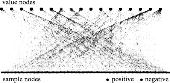
data simultancously.

Wc bricfly outline how to construct our visual classifier from

a

set $S$ of samplcs

on a

domain

$\mathcal{D}_{1}\cross\cdots\cross \mathcal{D}_{n}$ of $n$ attributes. We first represent the rclationship bctwccn $S$ and the domain as

a

two-layercd drawing of a bipartitc graph,

as

shown in Figurc 1, whcre each value node in thc

top lcvcl represcnts

one

of the values in $n$ attributcs, and each sample node in the bottom lcvcl

rcprcsenting

one

of thc samples is joincd by edges to the value nodes that specifies the saniplc.

We thcn try to rcduce the number of edge crossings bychanging thc drawing (i.e., the ordering

of nodes

on

each side) and by replacing two subdomains into their product

as a

ncw subdomain

(increasing the number of valuc nodes) until

a

tcrmination criteria is satisficd. Figure 2 shows

an example of

a

two-laycred drawing of

a

final bipartite graph, where

a

large number of positive

(negativc) samples form a cluster in the bottom levcl.

Wc

can

use

the resulting drawing

as

a classificr

as

follows. Given

a

new

samplc,

we

determine its

position in thc bottom level

as

the average of the positions of the corresponding valuc nodes, and

thcn judgc it

as

positive (negative) ifit falls amongpositive (negative) sample nodes. Performance

ofclassificr is usually evaluatcd by

error

rate

on

test sample set, and surprisingly,

our

classificr is

compctitive with a wcll-known decision trec classifier C4.5 [11].

This paper is organized

as

follows. We give the formal definition of bipartitc graphs, called

$’$

value

nodes

sample

nodes

$\bullet$

positive

$\bullet$

negative

Figure 1: The initial SF-graph from MONKS-I

niinimization algorithm for combining subdomains and permuting orderingsofnodes in SF-graphs

in Section 3. In Section 4,wc show how to

use

visualized SF-graphs as a

new

classifier. Wc prcsent

somc cmpirical studies in Section 5 and make concluding remarks in Scction 6.

2

Preliminary

2.1

Samples

and

Features

over

Attributes

III thc subsequent discussion, _{we assume} that a set $S=\{s_{1}, \ldots , s_{\pi\iota}\}$ ofpositive/ncgative samples

over

$n$ attributes is givcn. Let $\mathcal{D}_{j}$ denote thc domain ofattribute$j$, i.e., the set of allvalucs takcn

as a value of attributc $j$, wherc we

assume

that each $\mathcal{D}_{j}$ is

a

finite unordercd sct of at lcast two

discretc values. Each sample $s_{i}$ is spccificd by an n-dimensional vector $s_{i}=(s_{i.1}, s_{i,2}, \ldots, s_{i,n})$

such that $s_{i,j}\in \mathcal{D}_{j}$ for cach attribute $j\in\{1.2, \ldots, n\}$

.

Table 1 shows

a

set of six samples

over

4

attributes.

To handle subdomains of the entirc domain, wc dcfine “features” and “feature sets.” A

_feature

is a noncmpty subset $F\subseteq\{1,2, \ldots, n\}$ of the $n$ attributes, and thc domain $\mathcal{D}_{F}$ of a feature

$F=\{j_{1}, \ldots.j_{q}\}$ is dcfincd as the set of all combinations ofvalues taken by attributcs in $F$, i.e.,

$\mathcal{D}_{F}=\mathcal{D}_{j_{1}}\cross\cdots\cross \mathcal{D}_{j_{q}}$. The restriction $s|_{F}$ of

a

sample _{$s_{i}=(s_{i,1}, s_{i,2}, \ldots, s_{i,n})$} to featurc $F$ is

dcfincd by $(s_{i,j_{1}}, s_{i,j_{2}}, \ldots, s_{i,j_{q}})\in \mathcal{D}_{F}$

.

A value $v\in \mathcal{D}_{F}$ is called covered if there is asample $s_{i}\in S$

with $s_{i}|_{F}=v$, and a feature $F$ is callcd covered if all values $v\in \mathcal{D}_{F}$ are covered. A

feature

set

$\mathcal{F}=\{F_{1}, \ldots, F_{p}\}$ is a set of disjoint featurcs. i.e.. $F_{k}\cap F_{k’}=\emptyset$ for $k\neq k’$

.

The set of all values in

the domains of features $F_{1}\ldots.,$$F_{p}$ is denotcd by $\mathcal{D}_{\mathcal{F}}=\mathcal{D}_{F_{1}}\cup \mathcal{D}_{F_{2}}\cup\cdots\cup \mathcal{D}_{F_{r}}$

.

2.2

SF-graphs

Given

a

fcature sct $\mathcal{F}=\{F_{1}, \ldots , F_{\nu}\}$,

we

represent the relationship bctween thc sample set $S$

and the set $\mathcal{D}_{\mathcal{F}}$ of valucs by sample-feature graph (SF-graph), which is a bipartite graph $G_{\mathcal{F}}=$

value

nodes

Figure 2: A final SF-graph for MONKS-I

Table 1: A sample set $S=\{s_{1}\ldots., s_{6}\}$ with $\mathcal{D}_{1}=\{0,1\},$ $\mathcal{D}_{2}=\{0,1,2\},$ $\mathcal{D}_{3}=\{T, F\}$ and

$\mathcal{D}_{4}=\{Y, N\}$

.

Each value $v\in \mathcal{D}_{\mathcal{F}}$ is represented by a nodc, callcd a value node in the first node set, and

each samplc $s_{i}\in S$ is rcpresentcd by a node, called a sample node in the second nodc set,

wherc $\backslash vc$ use the samc notation for nodes for simplicity.

.

A valuc node $v$ and a samplc node $s_{i}$ is joincd by an edge $(v, s_{i})\in \mathcal{D}_{F}\cross S$ if and only if

$s_{i}|_{F_{k}}=v$ for somc feature $F_{k}\in \mathcal{F}$

.

Tbus thc cdgc sct is givcn by

$E_{\mathcal{F}}=\{(v,$ $s_{i})\in \mathcal{D}_{\mathcal{F}}\cross S|s_{i}|_{F_{k}}=v$ for some $F_{k}\in \mathcal{F}\}$

.

If$\mathcal{F}$ is

a

singlcton

$\mathcal{F}=\{F_{1}\}$,

we

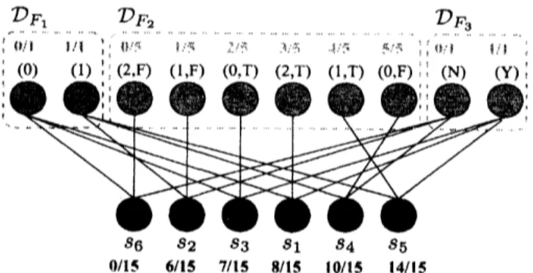
write $G_{\mathcal{F}}$ by $G_{F_{1}}$ for convenicnce.

Figurc 3 shows SF-graph $G_{F}=(\mathcal{D}_{\mathcal{F}}, S_{t}E_{\mathcal{F}})$ of thc sample sct $S$ in Tablc 1 for fcaturc sct

$\mathcal{F}=\{\{1\}, \{2,3\}, \{4\}\}$

.

The associated valuc vcctor is shown above each value node. Obscrvc that

SF-graph shows the membership of samples to the subdomains dctermined by features in $\mathcal{F}$

.

2.3

Visualization

by Two-Layered Drawings

We visualizc SF-graph $G_{\mathcal{F}}$with

a

two-layercd drawing, which is dcfincd by

a

pair of ordcrings

on

thc

$s_{1}$ $s_{2}$ $s_{3}$ $s_{4}$ $S_{5}$

Figurc 3: SF-graph $G_{\mathcal{F}}=(\mathcal{D}_{\mathcal{F}}, S, E_{\mathcal{F}})$ of the sample set $S$ in Table 1 constructed for $\mathcal{F}=$

$\{\{1\}, \{2,3\}, \{4\}\}$

For a set $\mathcal{F}$ of features, we dcnote an ordcring OIl the set $\mathcal{D}_{\mathcal{F}}$ of value nodes by a bijcction $\pi_{\mathcal{D}_{\mathcal{F}}}$ : $\mathcal{D}_{\mathcal{F}}arrow\{1, \ldots, |\mathcal{D}_{\mathcal{F}}|\}$

.

In thc rcst of the paper,

wc

abbreviate $\pi_{\mathcal{D}_{\mathcal{F}}}$ into $\pi_{\mathcal{F}}(\pi_{\mathcal{D}_{\mathcal{F}}}$ with

$\mathcal{F}=\{F_{k}\}$ into $\pi_{k}$) for convcnience if no confusion ariscs. In thc two-layercd drawing, the value

nodes in $\mathcal{D}_{\mathcal{F}}$ are placcd in the top level according to the order $\pi_{\mathcal{F}}$, while the sample nodcs in $S$

arc placcd in the bottom lcvel according to the order $\sigma$

.

Let $\chi(G_{\mathcal{F}}, \pi_{\mathcal{F}}, \sigma)$ denote the numbcr of

cdgc crossings in thc drawing $(\pi_{\mathcal{F}}.\sigma)$ of$G_{F}$

.

In order to find a “good” visualization of thc givcn samplc set $S$, we nccd to find a featurc sct

$\mathcal{F}=\{F_{1}, \ldots, F_{p}\}$ and its two-layered drawing $(\pi_{\mathcal{F}}, \sigma)$ such that $\chi(G_{\mathcal{F}}.\pi_{\mathcal{F}}, \sigma)$ is minimizcd

subject to

$F_{1}\cup\cdots\cup F_{p}=\{1,2,$ $\ldots\{n\}$,

each fcature $F_{k}\in \mathcal{F}$ is covered.

Thc motivation of this formulation is as follows. There

are

many graph drawing studics claiming

that cdgc crossings has the greatest impact

on

readability among various criteria (e.g., bends,

symmetry) [10, 6]. In terms of SF-graph, crossing minimization may provide

us

good inforination

on thc truc locations of samples in their domain which

wc

cannot usually

see.

Wcclaiin thatthc optimal ordering

on

sample nodes reflects their truc locations. This claim is

supported by the following observation: Let us take a feature set $\mathcal{F}$ having only

one

featurc. Wc

show how crossing minimization works for such $G_{\mathcal{F}}$ in Figurc 4. We observe that samples having

thc

samc

value (i.e., those belong to the

same

subdomain) get gathered together in a chain of

samples, which

we

call a sample chain,

as

the result of crossing minimization.

Note that merging two fcaturcs $F_{k},$ $F_{k}/\in \mathcal{F}$ into

a new onc

$F_{k’’}=F_{k}\cup F_{k^{l}}$ givcs a

two-layercd drawing with a smaller numbcr of edgc crossings. For

an

extreme example, the fcature set

$\mathcal{F}=\{F_{1}=\{1\ldots., n\}\}$ admits atwo-layercd drawing $(\pi_{\mathcal{F}}.\sigma)$ with no edge crossings, although $F_{1}$

is not covered in general (inmany data sets. it holdsthat $S\subseteq \mathcal{D}_{1}\cross\cdots x\mathcal{D}_{n}$). However, we

arc

not

interestcd in uncovered fcaturcs. Discarding suchoncs, thc number ofvalue nodes from a featurcof

our intcrcst is bounded by $m_{\dot{t}}$ while the domain ofa feature. direct product ofattributc domains,

can

be exponcntially large unlcss restrictcd. Sincc we havc

no

information

on

uncovered values,

Figurc 4: Crossing minimization

on

SF-graph with

one

feature

Hence

we can

expect that the above good visualizationidcntifies similarsamples and collccts thcm

as sample chains over a well-structurcd sct of subdomains.

2.4

Crossing

Minimization

We now revicw the studicson crossing minimization in two-laycrcd drawings. Two-sided crossing

minimization problem(2-CM) asksto dccideboth $\pi_{\mathcal{F}}$ and$\sigma$that minimize$\chi(G_{\mathcal{F}}, \pi_{\mathcal{F}}, \sigma)$

.

Howcver,

2-CM is NP-hard

evcn

if the ordering on one side is fixcd [4, 2, 7]. This restrictcd version of

2-CM is callcd one-sided crossing minimization problem (1-CM). We design a heuristic proccdure of

crossing minimization on SF-graph in the next section, whcre 1-CM with

a

fixcd ordcring on $\mathcal{D}_{\mathcal{F}}$

forms its bases. Thus, we can formalize 1-CM as follows.

Problem 1-CM$(G_{\mathcal{F}}, \pi_{\mathcal{F}})$

Input: A bipartite graph $G_{\mathcal{F}}=(\mathcal{D}_{\mathcal{F}}, S, E_{\mathcal{F}})$ and

an

ordering $\pi_{\mathcal{F}}$ on $\mathcal{D}_{\mathcal{F}}$

.

Output: An ordering $\sigma$

on

$S$ that niinimizes $\chi(G_{F}, \pi_{\mathcal{F}}, \sigma)$.

3

Algorithm

to Grow up SF-graph

In thissection, we dcscribe ouralgorithmPERMUTE-AND-MERGE for findinga goo$d’$visualization

of a givcn sample set $S$

.

It consists of two subroutines,

one

for combining two fcatures into

a

ncw

one, and the othcr for permuting value (samplc) nodes to reduce cdgecrossings. Note that replacing

tWO featurcs $F_{k}$ and $F_{k’}$ with thcir union $F=F_{k}\cup F_{k}$ノ increascs the number of value nodcs and

dccrcascs the numbcrofedges in SF-graph$\dagger$ since

$|\mathcal{D}_{F}|=|\mathcal{D}_{F_{k}}|\cross|\mathcal{D}_{F_{k}},$$|$ is larger than

$|\mathcal{D}_{F_{k}}|+|\mathcal{D}_{F_{k}},$$|$

andtwocdgcs $(s_{i}, a)$ and $(s_{i}, b)$with$a\in \mathcal{D}_{F_{k}}$ and $b\in \mathcal{D}_{F_{k’}}$

arc

replaced with

a

single cdge$(s_{1}(a, b))$,

$(a_{j}b)\in \mathcal{D}_{F}$

.

Thus the algorithm grows up the valuc node sidc of SF-graph by combining fcaturcs

until

no

two fcatures $F_{k}$ and $F_{k’}$ generate

a ncw

covercd fcature $F=F_{k}\cup F_{k},$.

Algorithm PERMUTE-AND-MERGE is describcd in Algorithm 1. Thc algorithm starts from thc

sct $\mathcal{F}$ of _$n$ singleton features (line 2) and arbitrary orderings on value and samplc nodcs (line 3).

Then it itcratcs computing nodc orderings by crossing minimization (using procedurc PERMUTE

in line 5) and merging

an

appropriatcpair offeaturcs into

one

(usingfunction MERGE inline 6); if

no pairrcsults in

a

covcred feature, thenthealgorithm

tcrminates.

The ncxttwoscctions dcscribe

$\frac{A1gorithm1PERhIUTE-AND- L4ERGF_{\lrcorner}}{1:procedure}$

2. $\mathcal{F}arrow\{\{j\}|j\in\{1\ldots. , n\}\}$ $\triangleright G_{F}$ is constructed

3. $\pi_{\mathcal{F}},$$\sigmaarrow$ arbitrary orderings

on

$\mathcal{D}_{\mathcal{F}},$ $S$

4: repeat

5. PERMUTE

6. until MERGE outputs $no$

$7$: output $G_{\mathcal{F}}$ and $(\pi_{F}, \sigma)$ $8$. end procedure

$\frac{A1gorithm2PERMUTE-BY- LS}{9:procedure}$

$\iota 0$

.

repeat

11. $\pi_{\mathcal{F}}^{i_{l1}it}arrow\pi_{\mathcal{F}},$$\sigma^{init}arrow\sigma$

12. for all $\pi_{\mathcal{F}}’\in N(\pi_{\mathcal{F}})$ do

13: $\sigma’arrow 1- CM(G_{\mathcal{F}}, \pi_{\mathcal{F}}’)$

14. if $\chi(G_{\mathcal{F}}, \pi_{\mathcal{F}}’, \sigma’)<\chi(G_{\mathcal{F}}, \pi_{\mathcal{F}}, \sigma)$ then

15. $\pi_{\mathcal{F}}arrow\pi_{\mathcal{F}}’,$ $\sigmaarrow\sigma’$

16. break the for-loop

17. end if

18: end for

19. until $\pi_{\mathcal{F}}\equiv\pi_{\mathcal{F}}^{init}$ and $\sigma\equiv\sigma^{init}$

20. end procedure

3.1

Procedure PERMUTE

The subroutinc PERMUTE can be any algorithm for crossing minimization. Here we proposc

PERMUTE-BY-LS in Algorithm 2,

a

hcuristic niethod based

on

local search. Starting from an

ordcring$\pi_{\mathcal{F}}$, thc local scarch sccks for a bettcr ordcring$\pi_{\mathcal{F}}’$ in its neighborhood. The neighborhood

of$\pi_{\mathcal{F}\tau}$ denotcd by $N(\pi_{\mathcal{F}})$

.

is a sct of ordcrings which

can

be obtained by

a

slight change of $\pi_{\mathcal{F}}$

.

A

ncighbor ordering $\pi_{\mathcal{F}}\in N(\pi_{F})$ is cvaluated by edge crossings $\chi(G_{\mathcal{F}}, \pi_{\mathcal{F}}’, \sigma’)$ where $\sigma’$ is obtained

bysolving 1-CM$(G_{\mathcal{F}}.\pi_{\mathcal{F}}’)$ (lincs 13 and 14). If thc edge crossings is smaller than the prcvious one.

then the proccdure adopts $\pi_{F}’$ and $\sigma’$ (line 15) and continues to scarch the neighborhood of thc

new $\pi_{\mathcal{F}}$. Othcrwisc, the proccdurc terminates.

Thc followings

arc

dctailcd scttings ofPERMUTE-BY-LS.

Restriction on Value Node Ordering. In order to rcduce the search spacc, wc rcstrict

our-sclves to such $\pi_{F}$ wherc valuc nodcs from thc samc fcature

are

ordered consccutivcly,

as

in

Fig-ure 3. This rcstriction cnablcs us to reprcsent $\pi_{\mathcal{F}}$

as

a concatenation of$p$ ordcrings $\pi_{1},$_$\ldots,$$\pi_{p}$ on

$\mathcal{D}_{F_{1}},$$\ldots.\mathcal{D}_{F},,$, wherc theconcatenation is givcn by

an

ordering $\pi^{*}$ : $\mathcal{F}=\{F_{1}, \ldots , F_{p}\}arrow\{1\ldots.,p\}$

.

Thus $\pi_{F}(v)$ for $v\in \mathcal{D}_{F_{k}}$ is given by:

Figure 5: SF-graph ordcrcd by thc barycenter heuristic

It is casy to show that the total number of edge crossings is given by:

$\chi(G_{\mathcal{F}},\pi_{\mathcal{F}}, \sigma)=\sum_{k=1}^{p}\chi(G_{F_{k}}, \pi k\cdot\sigma)$

$+p(p-1)|S|(|S|-1)/2$, (1)

whcre thc sccond termof the right hand is a constant for a fixcd$p$

.

The abovc cquality (1)

mcans

that thc nurnbcr of edge crossings is invariant with

a

choice of

an

ordcring $\pi^{*}$

on

$\mathcal{F}$. In what

follows,

we

conccntrate

on

searching $\pi_{1}\ldots.,$$\pi_{p}$ during the proccdure, assuming that $\pi^{*}$ is chosen

arbitrarily.

Neighborhood. For neighborhood $N(\pi_{\mathcal{F}})$,

wc

take the sct of all ordcrings

on

$\mathcal{D}_{\mathcal{F}}$ which

can

bc

obtaincd by swapping $\pi_{k}(v)$ and $\pi_{k}(v’)$ for any _$v,$$v’\in \mathcal{D}_{F_{k}}(k=1, \ldots,p)$

.

In line 12,

a

neighbor

$\pi_{\mathcal{F}}’\in N(\pi_{\mathcal{F}})$ is chosen at random.

Solving 1-CM. We usethc barycenter heuris$tic$in solving 1-CM$(G_{\mathcal{F}}, \pi_{\mathcal{F}}’)$to decide $\sigma$‘ in line 13

[14, 7]. Thc barycenter heuristic permutcs the set $S$ of sample nodes in the increasing ordcr of

barycenter valucs: Lct

us

takc any subsct$\mathcal{D}_{F_{k}}\subseteq \mathcal{D}_{\mathcal{F}}(k=1, \ldots ip)$

.

For

a

value node $v\in \mathcal{D}_{F_{k}}$ and

an ordcring $\pi_{k}’$ on $\mathcal{D}_{F_{k}}$,

we

define the normalized index$I(v.\pi_{k}’)$ as follows:

$I(v, \pi_{k}’)=\frac{\pi_{k}’(v)-1}{|\mathcal{D}_{F_{k}}|-1}$

.

(2)

Thc baryccntcr$\beta(s, \pi_{\mathcal{F}}’)$ of asample nodc $s\in S$ (w.r.t.

an

ordcring$\pi_{\mathcal{F}}^{l}$ on$\mathcal{D}_{\mathcal{F}}$ including$\pi_{1}’,$

$\ldots,$$\pi_{p}’$)

is defincd by

$\beta(s,\pi_{\mathcal{F}}’)=\frac{1}{p}\sum_{k=1}^{p}I(s|_{F_{k}}, \pi_{k}’)$

.

(3)

Figure5shows the rcsult of the barycentcr hcuristiconthcSF-graphofFigure 3, alongwith

nor-malizcd indicesofvalue nodcs and barycenter valucs of sample nodes. We note that$I(v, \pi_{k}’)=\pi_{k}’(v)$

is usually used in the literature to numbcr value nodcs. Howcvcr, by (2), all features have equal

influcncc in dcciding barycenter since $I(v, \pi_{k}’)\in[0,1]_{!}$

.

which improvcd the leaming performance

$\ovalbox{\tt\small REJECT}$ $\ovalbox{\tt\small REJECT}$

$l^{/\backslash }\bullet\backslash \cross^{/}$

$\chi=2,$ $\chi_{co1}=2$

$l^{/}b\ovalbox{\tt\small REJECT}_{\backslash _{\backslash _{\backslash }}}\ovalbox{\tt\small REJECT}\cross_{\backslash }^{/}$

$\chi=2,$ $\chi_{co1}=0$

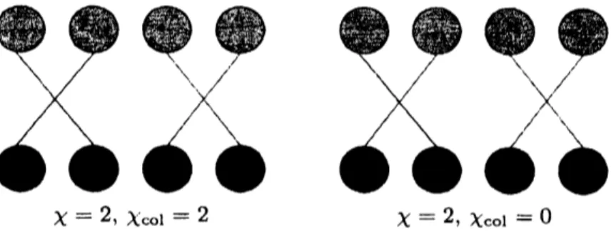
Figure 6: Illustration of$\lambda$ and $\chi_{co1}$

Evaluation of Orderings. In linc 14, it is natural to

usc

the number of edge crossings $\chi$ in

cvaluation of orderings $(\pi_{\mathcal{F}}, \sigma)$, but

we can

introducc various evaluating functions thcre. For

cxamplc,

assume

coloring each edge $(v, s_{i})\in E$ according to the class of sample $s_{i}\in S$

.

Then

we

can

dcfinc colored edge crossings $\chi_{co1}(G_{\mathcal{F}}, \pi_{\mathcal{F}}, \sigma)$ to be the number of crossings _{$be\{weendiIIerenl\downarrow$}

colorcd cdges. In thc two drawings in Figurc 6. $\chi_{co1}$ prefers the right one while $\chi$ rates both

situations similarly. By using $\chi_{co1}$

as an

evaluator. wc

can

cxpcct samplcs belonging to thc-

same

class to form clustcrs.

Analogouslywith$\chi$in(1), $\chi_{co1}(G_{\mathcal{F}}, \pi_{\mathcal{F}}, \sigma)$canbercprcscntcd

as

the summation of$\chi_{co1}(G_{F_{k}}.\pi_{k}.\sigma)$’s

and

a

constant. Takingthequalityoffcaturc intoaccount,wedefine weightedcolored edge crossings

$x_{co1}(G_{\mathcal{F}}.\pi_{\mathcal{F}}, \sigma)$ by

$\chi_{co1}^{*}(G_{\mathcal{F}}, \pi_{\mathcal{F}}, \sigma)=\sum_{k=1}^{p}\frac{\chi_{CO}l(G_{F_{k}}.\pi k\cdot\sigma)}{\rho(F_{k})}$ (4)

for an $impu7nty$

function

$\rho(F_{k})$ on $\mathcal{D}_{F_{k}}$ which indicatcs thc quality of feature $F_{k}$

.

Wc

use

thc

following for our cxperimcnts:

$\rho(F_{k})=\sum_{v\in \mathcal{D}_{F_{k}}}\deg^{+}(v)$dcg“(v),

wherc dcg$+(v)$ _and $\deg^{-}(v)$ denotc the $n\iota unbcrs$ of positive and negativc sample nodcs $s_{i}\in S$

with $s_{j}|_{F_{k}}=v$, rcspectively. The$\rho(F_{k})$ becomcs small (resp., largc) if$F_{k}$ divides the samplcset $S$

into purc (rcsp.. impurc) subscts in the

sense

ofclass distribution and thus may (resp., may not)

have nicc information on classification. Then $\chi_{co1}^{*}$ in (4) must be much influcnccd by $\chi_{co1}$ of good

fcatures.

3.2

Function MERGE

The subroutine MERGE inAlgorithm 1 can be any functionthatoutputs eithcr yesor $no$according

to whcthcr thcre exists

an

appropriate pair offcatures to bc merged. It should also mergc such

a

pair into

a new

featurc if yes.

Wc present our algorithm MERGE-BY-PRIORITYin Algorithm 3. The algorithm first constructs

a

priority qucuc $Q$ for all pairs of features in $\mathcal{F}$ (line 22). The prioritization of feature pairs

dctermincs the ordering according to $\backslash vhicli$ thcy arc tested for mcrge, and wc will mention thc

$\overline{\frac{A1gorithm3MERGE-BY-\underline{P}\underline{RI}ORITY}{21:function}}$

22: $Qarrow a$ priority queue _{for all pairs offcatures in}$\mathcal{F}$

23: while $Q$ is not empty do

24: $\{F_{k}, F_{k’}\}arrow$dequeue$(Q)$

25: $Farrow F_{k}\cup F_{k’}$

26: if $F$ is covered then

27: $\mathcal{F}arrow(\mathcal{F}\backslash \{F_{k}, F_{k’}\})\cup\{F\}$

28: reconstruct $G_{\mathcal{F}}$ for the

new

$\mathcal{F}$

29: _initialize $\pi_{\mathcal{F}}$

30: $\sigmaarrow 1- CM(G_{\mathcal{F}}, \pi_{\mathcal{F}})$

31; return _yes

32: end if

33: end while

34:

return

$no$

$35$: end function

Thc algorithm

removes

the feature pair $\{F_{k}, F_{k’}\}$ from the head of $Q$ (opcration dequeue in

linc 24) and tests whether it can be mergcd undcr

our

criteria. If$Q$ becomes empty

as

the result

of repetition of removal, then the algorithm retums $no$, indicating that there is no appropriate

feature pair to be merged.

Wc test in line

26

whether the

new

$F$ merged _{$homF_{k}$} and $F_{k’}$ is covcred, i.e., all generated

value nodes in $F$

are

conmccted to sample nodcs in the reconstructcd SF-graph. For example,

starting from $\mathcal{F}=\{\{1\}, \{2\}, \{3\}, \{4\}\}$, the pair of featurcs

{2}

and

{3}

passes the test since all

rcsultingvalue nodcs

are

connected,

as

shown in Figures

3

or

5.

If the feature pair $\{F_{k}, F_{k’}\}$ passes the test, thcn the algorithm mcrges $F_{k}$ and $F_{k’}$ into

a new

featurc $F=F_{k}\cup F_{k’}$, reconstructs SF-graph, initializes $\pi_{\mathcal{F}}$ and $\sigma$ and rctums yes (lines 27 to 31).

Now lct

us

describe the details of the algorithm.

Prioritization of Feature Pairs. Merge of feature pair has great influence

on

the quality of

the final drawing. Hence

wc

should be careful in choosing the priority

measure

which decides thc

ordering for test. In

our

cxpcriments, wc give higher priority to such a pair $\{F_{k}, F_{k’}\}$ that has

a

smaller value in the following summation:

$\frac{\chi_{co1}(G_{F_{k}},\pi_{k},\sigma)}{\rho(F_{k})}+\frac{\chi_{co1}(G_{F_{k’}},\pi_{k^{J}},\sigma)}{\rho(F_{k},)}$, (5)

which

comes

from the definition of wcightcd colored edge crossings (4). We expcct the abovc

evaluator to rcfinefeaturcs following the sample ordering well (whichhavc small $\chi_{co1}$)

or

to

remove

impure features (whichhave large $\rho$).

Initialization ofValue Node Ordering. In line 29, for the

new

$\mathcal{D}_{\mathcal{F}}$,

wc

needto decide $\pi_{\mathcal{F}}$ so

that it

serves as a

good initial solution in thc next local scarch. Let

us

recall that $\mathcal{F}$ has $p-1$

fcatures and that $\pi_{\mathcal{F}}$ is determined by orderings

on

$p-1$ value node subsets.

We

now

describe how to choosc $\pi_{F}$ on the value node set $\mathcal{D}_{F}$ arising from thc

new

feature

Table 2; _{Summary ofdata sets from}

_UCI

_Repository

$\overline{Data|S|n}$

$\overline{MONKS- 11246}$ MONKS-2 169 6 $\frac{MONKS- 31226}{BCW6999(22.6)}$

GLASS

214

9

(15.9) HABER 306 3 (34.4) HEART 270 13 (23.7) HEPA 155 19 (19.5)

IONO

200

34

(42.5)

found in the last local scarch,

we

decide $\pi_{F}$ by using lexicographic ordering based

on

them:

wc

definc $\pi_{F}(a)<\pi_{F}(b)$ for two valucs $a,$$b\in \mathcal{D}_{F}$ ifand only ifthe following holds:

$(\pi_{k}(a|_{F_{k}})<\pi_{k}(b|_{F_{k}}))$

or

$(\pi_{k}(a|_{F_{k}})=\pi_{k}(b|_{F_{k}})$ and $\pi_{k’}(a|_{F_{k}},)<\pi_{k’}(b|_{F_{k}}, ))$

.

Finally, we keep the orderings for the rest $p-2$ value node subsets which have not been changed

by merge.

4

Classifying with

Visualized

SF-graphs

In this section, we dcscribe how to use a two-layered drawing $(\pi_{\mathcal{F}}, \sigma)$ of a final SF-graph $G_{\mathcal{F}}$

as

a

new $\backslash ^{r}isua1$ classifier. Let

us

denote

a

test sample by $t\in \mathcal{D}_{1}\cross\cdots\cross \mathcal{D}_{n}$

.

Wc classify $t$ according

to its ncarest neighbor in barycenter: we examine the value nodcs to which sample node $t$ should

bc conncctcd, i.e., the value node $v\in \mathcal{D}_{F_{k}}$ with $t|_{F_{k}}=v$ for cach feature $F_{k}$ $(k=1, \ldots , p)$, and

compute its baryccntcr $\beta(t.\pi_{\mathcal{F}})$ by (3). Finally, we classify $t$ into the class of the nearest sample

in terms of barycentcr.

For cxample, lct

us

take the SF-graph in Figure 5 again. In this case, a test sample $t=$

$(1,2, F, Y)$ has baryccnter 10/15 and isclassified into negative class since negative sample $s_{4}$ is the

nearcst.

5

Empirical

Studies

In thissection, wepresentcmpiricalstudicsondatasets fromUCIRepository of Machine Leaming

[1]. First

we

give summary ofthe datasets, and then dcscribe cxperimentalresults.

5.1

Data

Sets

Table 2 shows the summary of the used data sets, whcre

we

will explain the decimals in the

rightmost column later. MONKS-I to 3

are

_artificial

data sets in the

sense

that theoraclc function

value nodes

sample nodes

$\bullet$

positive

$\bullet$

negative

Figurc 7: SF-graph obtaincd from MONKS-2

4 categorical valucs

as

its domain $\mathcal{D}_{j}$

.

For cxample,

a

sample $s_{i}=$ $(s_{i,1}, \ldots , s_{\dot{r},6})$ in MONKS-I is

positivc ifand only if $(s_{i,1}=s_{i,2})$

or

$(s_{i,5}= 1" )$

.

Thc othcrs

arc

real data scts, whcrc thc oraclc is not availablc. For examplc, BCW

(abbrcvia-tion of breast-cancer-wisconsin) consists of699 samples (paticnts), whcre 241 samples are positivc

(malignant) and thc rcst 458 samplcs

arc

ncgative (benign). Each samplc has intcgral valucs for 9

attributcs (c.g., clump thickncss, uniformity of ccll sizc).

Wc cvaluatc

a

classificr by its prcdiction

crror

rate

on

futurc samplcs. In thc litcraturc,

prcdic-tion

crror

ratc is usually cstimatcd by constructing

a

classificr from

a

training set of samplcs and

thcn cvaluating its

crror

ratc

on a

test set, _{For artificial data} scts,

we

takc thc cntirc data sct

as

the training sct and consider all possiblc samplcs

as

thc tcst sct by gcncrating them. The tcst sct

contains 432 samplcs in all for cach MONKS data sct.

For rcal data scts,

wc

cstimatc prcdiction

error

ratc by the avcrage of

crror

ratcs observcd in 5

trials of10-fold

cross

validation, awcll-known mcthodology to dividcthc datasct into training and

tcst scts. In thcsc data sets,

somc

attributcs takc continuous numcrical valucs which cannot bc

trcated in ourformulation. Thus wc gcncratc binarizationrulcs (e.g., arule may map a continuous

valuc to 1 ifit is larger than acomputcd thrcshold, and to $0$ otherwisc) from atraining sctby thc

algorithm proposcd in [5], and then construct

a

classifier from thc binarizcd data set. A decimal

in Tablc 2 indicatcs

avcrage

on

thc numbcr of gcncratcd binary attributcs.

5.2

SF-graphs

Figurcs 2 and 7 show thc output SF-graphs for MONKS-I and 2 respectivcly. Thc samplc chain

cxtractcd from thc output SF-graph for BCW is shown in Figurc 8. In all figurcs, wc

sce

that

samplcsofthc

samc

class fomiclustcrs. WcshowhowSF-graph providcs information in interactivc

data analysis.

MONKS-I. Among samplcs rcmotc from boundarics ofclustcrs,

wc

find thosc bclongingto thc

class to

a

strong dcgrcc:

a

samplc in MONKS-I is positivc ifand only ifit satisfies either condition

statcd in thc last subscction. Lct us rcgard thosc satisfying both conditions

as

strongly positivc

Figurc 8: Samplc chain from

BCW

and thc numbcr of $1$’s in samplc vcctor $\frac\frac{Tab1e3:Prcdictioncrrorratcs(\%)}{DataSFCC4.5,MONKS- 1l6.200.00}$ MONKS-2 25.60 29.60 $\frac{MONKS- 319..360.00}{BCW5.12\pm 0535.16\pm 0.64}$ GLASS $9.86\pm 0.94$ $7.74\pm 1.63$ HABER $38.30\pm 1.69$ $25.50\pm 1.16$ HEART $26.07\pm 1.11$ $21.31\pm 1.60$ HEPA $23.54\pm 2.03$ $20.89\pm 1.52$ IONO $20.20\pm 1.50$ $14.40\pm 1.08$

actually gathcrcd in thc lcft cnd of thc samplc chain.

MONKS-2.

Wc

scc

that similar samplcs gct closcr in tlic samplc chain: roughly spcaking,

wc

scc two largc clustcrs of positive samplcs in Figurc 7. A samplc $s_{i}$ in MONKS-2 is positive ifand

only if$s_{i}$ has nominal “1” for cxactly two attributcs. We obscrvcd that thc right clustcr contains

all positivc samplcs having nominal く1” _{for thc l-st attribute, and that thc lcft clustcr contains}

morc

than 70% ofpositivc samplcs (20 out of28) _{having nominal} “1” for thc 5-th attributc.

BCW. Figurc 8 shows the numbcr of l’s in binarizcd samplc vcctor by grccn linc bcsidcs the

obtaincd samplc chain. Bascd

on

our rcsearch cxpericncc, wchavc obscrvcd that samples

arc morc

likcly to bc positivc with many $1$’s although

wc

do not know thc oraclc function of BCW cxactly.

Wc can vicw the phenomena in _{the figure, wherc degrce of class mcmbcrship is also rcflectcd in}

thc samplc chain.

5.3

Classification

Wc construct an SF-graph bascd classifier (SFC for short)

as

described in Scction 4. Wc prcscnt

prcdiction

crror

ratcs in Tablc 3, whcrcwc comparc our SFC with C4.5 [11], awcll-known dccision

of 10-fold

cross

validation. C4.5 constructs dccision trccs within 1 sccond in all

cascs

whilc SFC

takcs from 1 (for GLASS) to 120 scconds (for IONO), which is not too cxpcnsivc. Wc obscrved

that computation timc of SFC is proportional to thc numbcr of attributcs which decidcs thc sizc

of neighborhood in thc local scarch. All cxpcrinicnts

are

conductcd

on our

PC carrying 2.$83GHz$

CPU

and $4GB$ _main

mcmory.

A typical decision trec is rcgardcd

as

disjunction of if-thcn mlcs, cach of which is rcprescnted

by conjunction ofconditions on oneattributc value. We canrcalizc small dccision trccs casily that

rcprcscnt thc oraclc functions of MONKS-I (scc Scction 5.1) and 3. and thus it is rcasonablc to

say that C4.5 is succcssful for the two data sets. On thc othcr hand, it must bc not bc

so

casy to

reprcscnt thc oraclc of

MONKS-2

(scc Scction 5.2) by small trcc, and for such

a

data set,

SFC

is

supcrior to C4.5.

Lct

us

discuss

our

results for rcal data scts. Our SFC is

worsc

than

C4.5

for alinost all thc

datasets but is competitivewith BCW. Thus SFC can attainsufficient classifiers for suitable data

sets. We nccd to further cxaminewhat data typc is suitable for SFC, but for such data sets. SFC

surcly

scrves as an

cxccllcnt classificr.

6

Concluding

Remarks

Our rcsults

arc

significant particularly in thc following

scnse:

for machine leaming rcscarch, our

cl assifier$is$ quitedifferent frorn existii_{$\iota gappi_{odt}$}}$[es$because it isconstructedbasedoncoinbiitatorial

formulation

(bipartitcgraphand crossingminimization) rather thangcomctric conccpts. Wc assert

that dccision trce is also

onc

of gcomctric classifiers sincc

a

typical algorithm constructs a dccision

trce by partitioning thc samplc domain with hyperplancs,

cvcn

though it is rcprcscntcd by trcc

on

thc surface. Thus

our

work may givc

a

ncw

dircction to studics of lcarning problems. For

information visualization,

on

thc othcr hand,

wc

could show possibilityof such

a ncw

schcmc that

cnablcs human to gain knowlcdgc using visualization.

It

socms

possiblc for us to improvc the pcrformancc of ourSFC classificr furthcr. For cxamplc,

wc may dividc a valuc nodc by thc currcnt definition into a pair of positivc and ncgativc valuc

nodcs, whcrc positivc (rcsp., ncgativc) samplc nodcs arc connccted to thc former (resp., lattcr)

ones.

This $sc1.1ing$ enlarges tlio search $\backslash sp_{\dot{c}}\iota c(\backslash$, but, wc think

$1_{\Sigma}haf$_, it $sho\iota ild$ be eSTcctivc for

our

purposc. Our futurework also includcs finding good application

areas

of

our

methodology togain

somc

niore insights from thc fccdback.

This work is supportcd by

Grant-in-Aid

for Young Scicntists (Start-up, 20800045) from Japan

Socicty for thc

Promotion

of

Sciencc

(JSPS).

References

[1] _{A. Asuncion and D.J. Newman. UCI Machine Leaming} $Repositor^{v}y$

.

Univcr-sity of California, Irvinc, School of Information and Computcr Scicnccs, 2007.

http:$//www.$_{ics.uci. edu/mlearn/MLRepository.html.}

[2] P. Eades and N. C. Wormald. Edge crossings in drawings of bipartite graphs. Algorithmica,

Vol. 11, pp. 379-403, 1994.

[3] J. H. Fricdman. Rccent advanccs in prcdictivc (machinc) lcarning. Joumal

_of

Classification,

[4] M. R. Garcy and D. S. Johnson. Crossing numbcr isNP-complctc.

SIAM

Joumal

on

Algebraic

and Discrete Methods, Vol. 4, pp. 312-316, 1983.

[5] K. Haraguchi and H. Nagamochi. Extcnsion of ICF classificrs to rcal world data scts. In

$IEA/AIE$, Vol,

₄₅₇₀

_{of Lecture Notes in ComputerScience, pp. 776-785, Kyoto, Japan, 2007.}

Springcr.

[6] W. Huang, S. Hong, and P. Eades. Layout effects on sociogram perception. In Proceedings

_of

Graph Drawing 2005 (GD2005), pp. 262-273, Limcrick. Ircland, 2006.

[7] M. J\"unger and P. Mutzel. 2-laycr _{straightlinc crossing minimization: Pcrformancc of cxact}

and

hcuristic

algorithms. Joumal

_of

Graph Algornthms and Applications, Vol. 1,

No.

1, pp.

1-25, 1997.

[8] Jon R. Kettcnring. Thc practice of cluster analysis. Joumal

_of

Classification, Vol. 23, pp.

3-30, 2006.

[9] R. S. Michalski, J. G. Carbonell, and T. M. Mitchcll. Machine Learning: An

_Artificial

Intel-ligence Approach. Morgan Kaufmann, 1983.

[10] H. Purchase. $W\}_{1}ic\dagger\iota$ aesthetic has the greatest effect

$0\iota|$ human understatiding? Trl Procecdings

of

the 5th Intemational

_Conference

on

Graph Drawing (GD’97), pp. 248-261, Romc, Italy,

1997.

[11] J. R. Quinlan.

_C4.5:

Programs

_for

Machine Leaming. Morgan Kaufmann,

1993.

[12] B. D. Ripley. Pattern Recognition and Neural Networks. Cambridge Univcrsity Prcss, 1996.

[13] B. Sch\"olkopf and A. J. Smola. Leaming with Kemels. MIT Press, 2002.

[14] _{K. Sugiyama, S. Tagawa, and M. Toda. Mcthods for visual undcrstanding of hicrarchical}

systcm structurcs. IEEE Transactions on Systems, Man, and Cybemetics, Vol. SMC-II,

No. 2, pp. 109-125, 1981.

[15] T. Tamura and T. Akutsu. Subccllular location prcdiction of proteins using support vector

machincs _{with alignmcnt of block scqucnccs utilizing amino acid composition. BMC}

Bioin-formatics.

Vol. 8, No. 466, Novcmber 2007.

[16] V. N. Vapnik. The Nature

_of

Statistical

Leaming Theory. Springcr, 2nd cdition, 1999.

[17] T. Washio and H. Motoda. Statc of thc art of graph-bascd data mining. ACM SIGKDD

Explorations Newsletter, Vol. 5, No. 1, pp. 59-68, July 2003.

[18] S. M.

Wciss

and C. A. Kulikowski. Computer Systems that Learn:

_{Classification}

and

Predic-tion Methods

_from

Stattstics, Neural Nets, Machine Leaming, and Expert Systems. Morgan

Kaufmann, 1991.

[19] I. H. Wittcn and E. Frank. Data Mining: Practical machine leaming tools and techniques.