Domain Decomposition Method and Infinite-Precision Numerical Simulation (Nonlinear problems in industry, domain decomposition methods and numerical simulations)

(1)

Domain Decomposition Method and Infinite-Precision

Numerical Simulation

Toshiki TAKEUCHI (竹内敏己) and Hitoshi IMAI (今井仁司)

Faculty ofEngineering, University ofTokushima, Tokushima 770-8506, Japan.

(徳島大学工学部)

1 Introduction

(Domain Decomposition Method) has been popularin numerical simulation It

saves

CPU time and memory space. Moreover, balanced accuracy realized by suitable resolution

in each subdomains makes numerical simulation stable.

On the other hand, (Infinite-Precision Numerical Simulation) has been developed

recently[5]. It attains ultimatelyhigh accuracy. From this property IPNS hasreclaimed new

fields of numerical simulation, e.g. direct simulation of inverse problems[3, 4, 6, 7].

In the paper application of DDM and IPNS is considered. Atest problem is solved.

Numerical results

are

investigated from the view point ofaccuracy.

2Application of DDM and IPNS

2.1 Infinite-Precision

Numerical

Simulation

Numerical

errors

originate from the truncation

error

in the discretization and the rounding

error.

Realization of highly accurate numerical simulation needs arbitrary reduction ofboth

errors.

For such numerical simulation

we

proposed asimple method called

IPNS(Infinite-Precision Numerical Simulation). IPNS consists of the arbitrary order approximation and

the multiple-precision arithmetic. The former is used for the arbitrary reduction of the

truncation

error.

The last is used for the arbitrary reduction of the rounding

error.

As

for the arbitrary order approximation spectral methods

are

very useful[l]. Especially, the

spectral collocation method is most useful. Its application is same in FDM, so it is easily

applicable to nonlinear problems,

even

to free boundary problems[10]. In the spectral

coll0-cation method, the order ofapproximation

can

be controlled by the number of collocation

points. The multiple-precision arithmetic[8] is

now

easily available. Alot of subroutines

about it

are

already prepared. Some libraries

are

free and distributed

on

the net, e.g

数理解析研究所講究録 1288 巻 2002 年 102-107

(2)

http:$//\mathrm{w}\mathrm{w}\mathrm{w}$.lmu.$\mathrm{e}\mathrm{d}\mathrm{u}/\mathrm{a}\mathrm{c}\mathrm{a}\mathrm{d}/\mathrm{p}\mathrm{e}\mathrm{r}\mathrm{s}\mathrm{o}\mathrm{n}\mathrm{a}\mathrm{l}/\mathrm{f}\mathrm{a}\mathrm{c}\mathrm{u}\mathrm{l}\mathrm{t}\mathrm{y}/\mathrm{d}\mathrm{m}\mathrm{s}\mathrm{m}\mathrm{i}\mathrm{t}\mathrm{h}2/\mathrm{F}\mathrm{M}\mathrm{L}\mathrm{I}\mathrm{B}$.html [9]. IPNS has bee

applied to many problems and ultimately high accuracy has been

seen

in numerical results.

2.2 Test

problem

We consider the following simple boundary value peoblem.

Problem 1. For agiven $a$ find $u(x)\mathrm{s}.\mathrm{t}$.

$\{$

$\frac{d^{2}u}{dx^{2}}=\frac{-8a^{2}(e^{ax}-e^{-ax})}{(e^{ax}+e^{-ax})^{3}}$,

$-1<x<1$

,

$u(-1)= \frac{e^{-a}-e^{a}}{e^{-a}+e^{a}}$, $u(1)= \frac{e^{a}-e^{-a}}{e^{a}+e^{-a}}$.

(1)

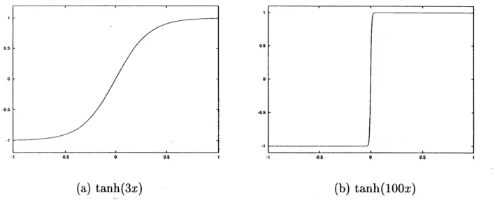
Remark 1. The exact solution to Problem 1is $u(x)= \tanh(ax)=\frac{e^{ax}-e^{-ax}}{e^{ax}+e^{-ax}}$.

If

$a$ is

large this problem becomes

_difficult

to be solved numerically. This is because

_for

a large $a$ the

solution becomes the step

_function

approximately. This situation can be seen in Fig. 1.

(a) $\tanh(3x)$ (b) $\tanh$(100x)

Fig. 1. Exact solutions for various values of $a$.

2.3 Application

of DDM and IPNS

The exact solution to Problem 1is analytic, so IPNS can catch it in arbitrary accuracy.

However, if $a$ is large, IPNS cost very much. Thus efficiency of DDM to such acase is our

interest. Our interest is rather mathematical,

so

parallel computing or automatic domain

decomposition are not considered. DDM is applied to Problem 1as follows. The domain

103

(3)

is decomposed into three subdomains [-1, -c], [-c, c] and [c, 1] where

_$0<c<1$

. Then

Problem 1is decomposed into the following three problems.

$\{$ $\frac{d^{2}u}{dx^{2}}=\frac{-8a^{2}(e^{ax}-e^{-ax})}{(e^{ax}+e^{-ax})^{3}}$, $c<x<1$, $u(1)= \frac{e^{a}-e^{-a}}{e^{a}-e^{-a}}$, (2) $\frac{d^{2}u}{dx^{2}}=\frac{-8a^{2}(e^{ax}-e^{-ax})}{(e^{ax}+e^{-ax})^{3}}$,

$-c<x<c$

, (3) $\{$ $\frac{d^{2}u}{dx^{2}}=\frac{-8a^{2}(e^{ax}-e^{-ax})}{(e^{ax}+e^{-ax})^{3}}$,

$-1<x<-c$

, $u(-1)= \frac{e^{-a}-e^{a}}{e^{-a}+e^{a}}$. (4)

For the application of IPNS _{with the Chebyshev polynomial in each subdomains, the}

fol-lowing mapping functions

are

indroduced for mapping each subdomains into [-1, 1]. For

$-1\leqq t\leqq 1$

$\{\begin{array}{l}x_{1}(t)=\frac{\mathrm{l}-c}{2}(t+1)+cx_{2}(t)=ctx_{3}(t)=\frac{1-c}{2}(t+1)-1\end{array}$ (5)

By using these mapping functions equations in subdomains

are

transformed

as

follows,

re-spectively. $\{\begin{array}{l}\frac{d^{2_{4}}\tilde{u}_{1}}{dt^{2}}=\frac{-2a^{2}(\mathrm{l}-c)^{2}(e^{ax_{1}(t)}-e^{-ax_{1}(t)})}{(e^{ax_{1}(t)}+e^{-ax_{1}(t)})^{3}}\tilde{u}_{1}(1)=\frac{e^{a}-e^{-a}}{e^{a}+e^{-a}}\end{array}$

$-1<t<1$

, (6) $\frac{d^{2}\tilde{u}_{2}}{dt^{2}}=\frac{-8a^{2}c^{2}(e^{act}-e^{-act})}{(e^{act}+e^{-act})^{3}}$,

$-1<t<1$

, (7)

104

(4)

$\{$

$\frac{d^{2}\tilde{u}_{3}}{dt^{2}}=\frac{-2a^{2}(1-c)^{2}(e^{ax_{3}(\mathrm{t})}-e^{-ax_{3}(\mathrm{t})})}{(e^{ax_{3}(t)}+e^{-ax_{3}(t)})^{3}}$,

$-1<t<1$

,

$\tilde{u}_{3}(-1)=\frac{e^{-a}-e^{a}}{e^{-a}+e^{a}}$.

(8)

Here $\tilde{u}_{i}(t)=u(x_{i}(t))$, $i=1,2,3$. As for patching conditions the followings

are

introduced :

$\{$ $\tilde{u}_{1}(-1)$ $=\overline{u}_{2}(1)$, $\frac{d\tilde{u}_{1}}{dt}(-1)$ $= \frac{1-c}{2c}\frac{d\tilde{u}_{2}}{dt}(1)$, (9) $\{$ $\tilde{u}_{2}(-1)=\tilde{u}_{3}(1)$, $\frac{1-c}{2c}\frac{d\tilde{u}_{2}}{dt}(-1)=\frac{d\tilde{u}_{3}}{dt}(1)$. (10)

As mentioned before, our interest is efficiency of DDM in accuracy. So, iteration for parallel

computing is not used. Eqs. (6), (7), (8), (9) and (10) are discretized by SCM(Spectral

Collocation Method) with the Chebyshev polynomial and C-G-L(Chebyshev-Gauss-Lobatto)

collocation points and they are solved simultaneously in high precision. Multiple precision

arithmetic is not necessary in numerical computation seen later.

3Numerical Results

In this section numerical results are shown. Oursimpleinvestigation did not require multiple

precision and consequently strict IPNS

was

not carried out. However, results obtained here

suggest the role of DDM in IPNS. Of course, IPNS is necessary for detailed investigation.

For the case where DDM is not applied, i.e. Problem 1is solved by IPNS without DDM,

$(N+1)$ C-G-L points in [-1, 1] are used. Then,

error $= \max 0\leqq j\leqq N|u^{c}(x_{j})-u(x_{j})|$, $x_{j}= \cos\frac{j\pi}{N}$, $\dot{\gamma}=0,1$,$\cdots$ , $N$, (11)

where $u^{c}$ and _$u$ denote the numerical solution and the exact solution, respectively. For

the case where DDM is applied, $(N_{1}+1)$, $(N_{2}+1)$ and $(N_{3}+1)$ C-G-L points are used

in $[c, 1]$_, $[-c, c]$, and $[-1, -c]$, respectively. Then, $N=N_{1}+N_{2}+N_{3}$. Moreover, $N_{1}=N_{3}=10$ for our purpose. Then,

error $= \max\{\max 1\leqq i\leqq 30\leqq j\leqq N_{i}|\overline{u}_{i}^{c}(t_{j}^{i})-u(x_{i}(t_{j}^{i}))|\}$, $t_{j}^{i}= \cos\frac{j\pi}{N_{i}}$,

$\dot{J}$

(5)

$\prime ic$ denotes the numerical solution by DDM.

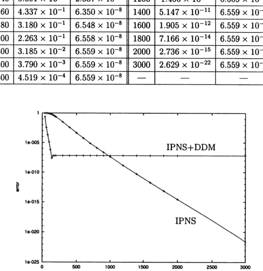
Table 1. Maximum

error

for Problem 1with $a=1\mathrm{O}\mathrm{O}$.

(Quadruple precision, DDM : $c=0.1$, $N_{1}=N_{3}=10$)

$\overline{\mathrm{Q}\mathrm{g}}$

Fig. 2. Behavior of maximum

error

for Problem 1with $a=1\mathrm{O}\mathrm{O}$.

(Quadruple precision, DDM : $c=0.1$, $N_{1}=N_{3}=10$)

1these numerical results it is

seen

DDM is efficient in IPNS. This

means

DD

space (and CPU time) for adegree of accuracy comparing with the case 1

(6)

not used. At the

same

time, _{it should be remarked} improper DDM spoils merit of DDM. This means high resolution in theregion where solutions change alot does not always attain

high accuracy.

4Conclusion

In the paper DDM is applied in IPNS. Numerical results show efficiency of DDM

on

saving

memory space (and CPU time). At the

same

time they also show high accuracy is not

attained by improper resolution in each subdomains. Our future work is parallelization and

solving more difficult problems in high accuracy.

Acknowledgements

This work is partially supported byGrants-in-AidsforScientific Research (No. 13640119),

from the Japan Society of Promotion of Science.

References

[1] C. Canutoet al., Spectral Methods in Fluid Dynamics, Springer, 1998.

[2] N. Debit et al., Domain Decomposition Methods in Science and Engineering, ddm.org, 2001.

[3] H. Imai and T. Takeuchi, Application of the Infinite-Precision Numerical Simulation to

an.

Inverse

Problem, NIFS-PROC-40(1999), 38-47.

[4] H. Imai and T. Takeuchi, Some Advanced Applications of the Spectral Collocation Method, GAKUTO

Int. Ser. Math. Sci. Appl., 17(2001), 323-335.

[5] H. Imai, T. Takeuchi and M. Kushida, On Numerical Simulation ofPartial Differential Equations in Infinite Precision, Advancesin Mathematical Sciencesand Applications, $9(2)(1999)$, 1007-1016.

[6] H. Imai, T. Takeuchi, M. Nakamura and N. Ishimura, ADIRECT APPROACH TO AN INVERSE

PROBLEM, GAKUTO Int. Ser. Math. Sci. Appl., 12(1999), 223-232.

[7] H. Imai, T. Takeuchi andH. _{Sakaguchi, Infinite Precision Numerical Simulation} _for _{PDE Systems and} Its Applications, RIMS Kokyuroku, Kyoto University, 1147(2000), 42-50.

[8] D. E. Knuth, TheArt of Computer Programming,Addison-Wesley, 1981.

[9] D. M. Smith, AFORTRAN Package For Floating-Point Multiple-Precision Arithmetic, Transactions

on Mathematical Software, 17(1991), 273-283.

[10] Tarmizi, T. Takeuchi,_{H. Imai and M. Kushida, Numerical simulation of one-dimensional free boundary}

$\mathrm{p}\mathrm{r}.\mathrm{o}\mathrm{b}\mathrm{l}\mathrm{e}\mathrm{m}\mathrm{s}\cap\cap$ in infiniteprecision,Advancesin Mathematical Sciences andApplications, 10(2)(2000), 661