A mathematical model for a hysteresis appearing in adsorption phenomena (New developments of the theory of evolution equations in the analysis of non-equilibria)

(1)

A mathematical model for

a

hysteresis

appearing

in

adsorption phenomena

日本女子大学理学部愛木豊彦(Toyohiko Aiki)

Department of Mathematical and Physical Sciences, Faculty of Science

Japan Women’s University

名城大学理工学部村瀬勇介 (Yusuke Murase)

Department of Mathematics, Faculty of Science and Technology

Meijo University

長岡工業高等専門学校一般教育科佐藤直紀 (Naoki Sato)

Division of General Education

Nagaoka National College ofTechnology

千葉大学教育学部白川健 (Ken Shirakawa)

Department of Mathematics, Faculty of Education

Chiba University

1 Introduction

In the present paper we propose an original mathematical model for a hysteresis

ap-pearing in adsorption phenomena. The mathematical model (FBP) will be given in

Section 3

as

a free boundary problem, in which the free boundary stands between the

regions of moisture liquid and moisture vapor in one hole of a porous medium. The

aim of this paper is to contribute researches for complex systems including hystereses

through a discussion about a modeling process for the new mathematicaldcscription of

the hysteresis.

Our study is motivated to

overcome

difficulties that

arose

in the works for three

dimensional concrete carbonation process in [2, 3, 4]. In these papers a mathematical

model for the process

was

proposed and studied taking into account of a hysteresis

effect. The model consists of quasilinear diffusion equations with a hysteresis operator

approximately described by

a

type of

a

play operator which is given by an ordinary

differential equation including the subdifferential of the indicator function for a closcd

interval. Here, we note that the uniqueness question remains open in either of [2, 3, 4].

The difficulty of the uniqueness is caused by the fact that the continuous dependence

between a solution and given data of quasilinear parabolic equations is not sufficient

to conform to the continuous property of the play operator summarized as follows (see

[12, 22] for details):

$(*)$ For a play operator $\mathcal{P}$ : $C([O, T])arrow C([O, T])$ with $0<T<\infty,$

$|\mathcal{P}(v_{1})-\mathcal{P}(v_{2})|_{C([0,T])}\leq C|v_{1}-v_{2}|_{C([0,T])}$ for $v_{1},$ $v_{2}\in C([0, T])$,

(2)

When we consider the model for concrete carbonation, the input function$v$ of the

opera-tor is a solution of the quasilinear parabolic equation andthe output function $w=\mathcal{P}(v)$

appears in the coefficient of the equation. In most of quasilinear parabolic equations, it

is not easy to obtain an estimate for difference of solutions with respect to atopologyof

the space of continuous functions. Thus it is not easy to prove the uniqueness.

Inordertoovercome these difficulties wecan choose thefollowingtwo ways. Thefirst

way is toimprovecontinuous properties of solutions to thequasilinearparabolicequation.

The second

one

is to develop a new mathematical description of a hysteresis operator.

For the past years the mathematical treatment with the ordinary differential equations

was applied for thc study to various mathematical models for nonlinear phenomena.

Also, the following advantages of such a treatment were pointed out in [1]. One of

advantages is to approximate them easily and the other is to enable to describe change

of the hysteresis by perturbation of given data. However,

as

mentioned above this

treatment has aweakness

on

the continuous property. Moreover, for the treatment it is

hard to express a behavior inside of the hysteresis $10$op, because the treatment is just

a phenomenologically approach. Then, based on these arguments we choose the second

way

as

a strategy in this paper, and hence our main aim is to propose a new model for a

hysteresis appearing in adsorption process by consideration for a mechanism, in detail.

The discussion of this paper will be proceeded

as

follows. In the next Section 2,

we briefly

see

the hysteresis operators appearing in adsorption phenomena. Due to this

observation

our

original model (FBP) is statedin Section 3. In

Section

4

we

consider an

algorithm to obtain approximatesolution, and show some data of numerical experiments

associated with (FBP). Finally, in Section5, we comment about the adequacy of (FBP)

by taking into account the numerical data, and discuss about the future prospects.

2 Adsorption phenomenon

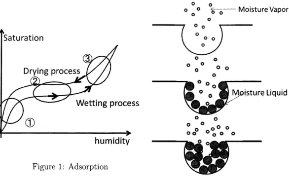
In this section we focus the relationship between the humidity and the saturation

de-scribing an adsorption phenomenon (see [16]). The hysteresis is a type ofinput-output

relationship between the humidity and the saturation in one hole of a porous medium.

From the experimental data (Figure 1)

we

have the following three features

on

the be-havior of the graph:

$\bullet$ Around $1$ and $3$ the slopes

are

steep.

.

Around $2$ the slope is gradual.

$\bullet$ The loop depends

on

the historical data.

The scenario for the behavior the relationship is described as follows (see Figure 2

to get general schcmes of the ideas): We consider one hole of the porous medium and

suppose that the degree of saturation

can

be regarded

as

the $vo$lume ratio of the liquid

in the hole. When the humidity is low, moisture vapor touches the wall directly and

becomes moisture liquid. After the surface ofthe wall is covered with moisture liquid, moisture vapor touches the liquid and becomes liquid.

Since

attractive force between

(3)

$\Diamond oc_{O}$

$oo\mapsto 0$ Moisture Vapor

Figure 1: Adsorption

Figure 2: Scenario of adsorption

slope will be gradual

as

the humidity becomes high. When the humidity rises further,

the slope becomes steeper, since the probability that the vapor touches the liquid in the

hole is also high,

Therefore, the aims of this research are to propose a mathematical model

represent-ing the above scenario and to confirm that the above graph obtained from numerical

simulations for the model.

3 Mathematical modeling for

adsorption

In this section we shall propose our mathematical model for adsorption phenomena.

First, we simplify a hole in the porous medium as one dimensional compact interval

$[0, L]$, where $L$ indicates the depth of the hole. Moreover, we assume that at $x=0$ the

wall exists, from the point $x=L$ the atmosphere flows into the hole, and the domain

$[0, L]$ is separated by the liquid region $(0, s)$ and the vapor region $(s, L)$ (see Figure 3),

Under these assumptions

we

define the degree of saturation $w$ by

$w= \frac{s}{L}.$

Inthis paperthe humidity$u=u(t, x)$ _{indicates the ratio of volume of moisture vapor}

per unit volume for any time $t$ and the spatial position $x$. Then the

mass

conservation

leads to

$\rho_{v}u_{t}+j_{x}=0$ in $(s, L)$,

(4)

Figure 3: One-dimensional model Figure 4: Near the free boundary

implies that $j=-\kappa u_{x}$ and

$\rho_{v}u_{t}-\kappa u_{xx}=0$ in $(s, L)$,

where $\kappa$ is a diffusivity constant.

Next, we consider the

mass

conservation of moisture near the free boundary $x=$

$s(t)$ for $t>0$ . If $s’(t)>0$ , then for small $\triangle t>0$ the

mass

of vapor of the interval

$(s(t), s(t+\triangle t))$ is given by

$\int_{s(t)}^{s(t+\Delta t)}\rho_{v}u(t, x)dx.$

Also, the

mass

of liquid

on

$(s(t), s(t+\triangle t))$ at time $t+\triangle t$ is given by

$\rho_{\tau v}(s(t+\triangle t)-s(t))$,

where $\rho_{w}$ is the density of moistureliquid (see Figure 4). Then. it holds that

$\rho_{w}(s(t+\triangle t)-s(t))=\int_{s(t)}^{s(t+\triangle t)}\rho_{v}u(t, x)dx-\Delta t\cross j(t, s(t+\triangle t))$,

and by letting $\triangle tarrow 0$

we

have

$\rho_{w}s’(t)=\rho$

。$s’(t)u(t, s(t))+\kappa u_{x}(t, s(t))$.

We note that the above equation also holds in

case

$s’(t)\leq 0.$

According to the scenario shown in the previous section the dynamics of the free

boundary depends on the distance between the wall and the front of the liquid region,

and the humidity at the front. Then we

assume

$s’(t)(= \frac{d}{dt}s(t))=\alpha(s(t), u(t, s(t)))$ for $t>0$, (3.1)

(5)

Here, from simple observations

we

can give some assumptions for $\alpha$. First, as the

humidity at the front is high, the vapor can easily become moisture liquid. This implies

$\frac{\partial}{\partial u}\alpha(s, u)>0$ for $(s, u)\in R^{2}$. (3.2)

Next, if the humidity is extremely high, then the front must grow. Also, if the humidity

vanishes, then thefront can not grow. Namely, for any $s\in R$ it should be that

$\alpha(s, u)\geq 0$ for $u\geq 1$ and $\alpha(s, u)\leq 0$ for $u\leq 0$. (3.3)

Moreover, since the front of liquid region can not grow beyond the gate of the hole and

the wall, we can suppose that for any $u\in R$

$\alpha(s, u)\leq 0$ for $s\geq L$ and $\alpha(s, u)\geq 0$ for $s\leq 0$_. (3.4)

Thus we have obtained the following free boundary problem (FBP) to find a pair

$\{s, u\}$ of a

curve

$x=s(t)$

on

$[0, T],$ $0<T<\infty$_, _and a_function $u=u(t, x)$ on $Q_{s}(T)$ $:=$

$\{(t, x)|s(t)<x<L, 0<t<T\}$ satisfying

$\rho_{v}u_{t}-\kappa u_{xx}=0$ in $Q_{s}(T)$, (3.5)

$u(t, L)=g(t)$ for

$0<t<T$

, (3.6)

$u(O, x)=u_{0}(x)$ for $s_{0}<x<L,$

$s’(t)=\alpha(s(t),$$u(t, s(t))$ _{for $0<t<T,$}

$\kappa u_{x}(t, s(t))=(\rho_{w}-\rho_{v}u(t, s(t)))\alpha(s(t), u(t, s(t)))$ for $<t<T$, (3.7)

$s(0)=s_{0},$

where $s_{0}$ is a initial position of the free boundary, and $g$ and $u_{0}$ are given boundary and

initial functions on $[0, T]$ and $[s_{0}, L]$, respectively. In [20] we establish the well-posedness

for the above problem under the assumptions (3.2) $\sim(3.4)$.

4 Numerical simulation

In this section we consider the problem (FBP) and present its numerical simulation.

First, we show the values ofconstants in (FBP)

as

the following Table 1:

$\frac{L\kappa\rho_{w}\rho_{v}s_{0}}{1111.73\cross 10^{-5}0.01}$

Table 1: Values ofconstants

Also, we set $u_{0}(x)=0$ for $x\in(s_{0}, L)$

.

Here,wegivetwo remarks concerned with anumerical simulationto (FBP)

as

follows:

1. (FBP) is a free boundary problemso that the domain $(s(t), L)$ _is_unknown for each

time $t$, where $\{s, u\}$ is asolution of (FBP). Moreover, since the value of$u(t, s(t))$

is also unknown, it is not easy to extend $u$

on

the fixed interval, for example $[0, L],$

(6)

2. There is

a

big difference between orders of $\rho_{v}$ and $\rho_{w}$. By this it takes

a

lot time

to calculate the solution, numerically. We

see

this property if the original domain

maps into cylindrical domain by change of variable, especially.

Hence, in order to solve these problems

we

develop the following algorithm for our

numerical simulations. For $\triangle t>0$

we

find approximations of$s(n\triangle t)$ and $u(n\triangle t, x)$ for

$n=1,2,$$\cdots$ , and $x\in(s(n\triangle t), L)$. As you

see

the algorithm, the number of latticc

points and the mesh size on space depend on $n$ so that we denote them by $N_{n}$ and

$(\triangle x)_{n}$ for each $n$. Thus

we

calculate $s_{n}$ and

$u_{n}^{(i)}$

as

approximations of $s(n\triangle t)$ and

$u(n\triangle t, s(n\triangle t)+i(\triangle x)_{n})$, respectively, for $n$ and $i=0,1,$$\cdots,$$N_{n}.$

Step 1. Set $n=0,$ $s_{n}=s_{0},$ $N_{n}=40$, and $u_{n}^{(i)}=u_{n}(s_{n}+i( \frac{L-s_{n}}{N_{n}}))$ for $i=0,1,$$\cdots,$$N_{n}.$

Step 2. Set $( \triangle x)_{n}=\frac{L-s_{n}}{N_{n}}.$

Step 3. Set $u_{n}^{(-1)}=u_{n}^{(1)}- \frac{2(\triangle x)_{n}}{\kappa}(\rho_{w}-\rho_{v}u_{n}^{(0)})\cross\alpha(s_{n)}u_{n}^{(0)})$.

Step 4. Put $s_{n+1}=s_{n}+\triangle t\cross\alpha(s_{n}, u_{n}^{(0)})$.

Step 5. Let $N_{n+1}’= \max\{j\in N|j\leq\frac{L-.s_{n+1}}{0025}\},$ $N_{n+1}= \max\{\min\{40, N_{n+1}’\}, 10\}$ and

$( \triangle x)_{n+1}=\frac{L-s_{n+1}}{N_{n+1}}.$

Step 6. Compute $\overline{u}^{(i)}$

from $u_{n}^{(i)}$ for $i=-1,0,1,$

$\cdots,$ $N_{n+1}$ by using the Lagrange

inter-polation with degree $1+N_{n+1}$, where $\overline{u}^{(i)}$

is corresponding to an approximation of

$u(n\triangle t, L-i(\triangle x)_{n+1})$

.

Step 7. Compute $u_{n+1}^{(i)}$ for $i=0,1,$

$\cdots,$$N_{n+1}$

as

an approximate solution satisfying

(3.5), (3.6) and (3.7) from $\overline{u}_{n}^{(i)}$

by using the Gauss-Seidel method.

Step 8. Set $n:=n+1$ and $GOTO$ _Step _2.

In order to verify the correctness of

our

algorithm

we

put

$s(t)= \frac{3}{4}(1-e^{-t})+\frac{1}{4}, u(t, x)=(1+\sin\pi x)e^{t},$

$\alpha(s, u)=(1+u^{2})(u-\frac{\arctan(l0s-6)-\arctan(-6)}{arc\tan(4)-\arctan(-6)})$ .

Then, $u$ and $s$ satisfy

$\rho_{v}u_{t}-\kappa u_{xx}=f$ in $Q_{s}(T)$,

$u(t, L)=g(t)$ for $0<t<T,$

$u(O, x)=u_{0}(x)$ $:=1+\sin\pi x$ for $s_{0}<x<L,$

$s’(t)=\alpha(s(t), u(t, s(t)))+k(t)$ for $0<t<T,$

$\kappa u_{x}(t, s(t))=(\rho_{w}-\rho_{v}u(t, s(t)))(\alpha(s(t), u(t, s(t)))+k(t))+h(t)$ for $<t<T,$

(7)

where $f(t, x)=(\rho_{v}+(\rho_{v}+\kappa\pi^{2})\sin\pi x)e^{t},$ $g(t)=e^{t},$ $k(t)= \frac{3}{4}e^{-t}-\alpha(s(t),$$u(t, s(t))$ and

$h(t)= \kappa\pi e^{t}\cos(\pi s(t))-\frac{3}{4}(\rho_{w}-\rho_{v}u(t, s(t)))e^{-t}$for $(t, x)\in Q_{s}(T)$ for $T>0.$

Since we know the exact solution of the above problem, we can calculate errors of

approximate solutions obtained by our algorithm and summarize these errors as the

following Table 2:

Table 2: Errors

From these results we infer that our method is somehow effective to (FBP). Then by

using this algorithm we obtain the following solutions.

$0\{$ $0$フ 03

$04\kappa’\backslash /)0^{r_{)}}$

, 0.$6$ 0.$7$ 0.$8$ 09 $0$ 01 $0.$? 03

$04t’\backslash t^{\backslash }0_{\backslash }\Gamma)$ 06

01 08 09

Figure 5: Simulation 1 Figure 6: Simulation 2

In Simulation 1 (Figures 5) we set

$\alpha(s, u)=(1+u^{2})(u-\frac{\arctan(l0s-6)-\arctan(-6)}{\arctan(4)-\arctan(-6)})$ , and $g(t)=\{$ $\frac{t}{25}-\frac{t}{5}$ $(5<t\leq 10)$, $(0<t\leq 5)$, $\frac{t}{5}-2$ $(10<t\leq 15)$, $4- \frac{t}{5}$ $(15<t\leq 19)$, $\frac{t}{5}-3.6$ $(19<t\leq 22)$, $5.2- \frac{t}{5}$ $(22<t\leq 24)$, $\frac{t}{5}-4.4$ $(24<t\leq 25)$, $5.6- \frac{t}{5}$ $(25<t\leq 26)$. (4.1)

Also, in Simulation 2 (Figures 6)

we

set

(8)

where

$\beta(u)=\{$ $\frac{o_{1-\cos(\pi u)}}{12}$ $ifu\in ifu<ifu>[0’, 1]01,$

’ $\gamma(s)=\{\begin{array}{ll}0 if s<0,\frac{1-\cos(\pi s)}{2} if u\in[0,1],1 if s>1,\end{array}$

$g$ is given by (4.1).

From observations these graphs in Figures 5 and 6 we can conclude that:

$\bullet$ Sincemost of the ascending branchesarelocated under descending ones, ourgraphs

are

quite similar to graphs obtainedbyexperiments. In this

sense we can

represent

the hysteresis in the absorption phenomena by (FBP).

.

Our graphs do not have the features mentioned in Section 2. More precisely, the

slopes for the low and high humidities are gradual in Figure 5 and the slope for

the low humidity is too, in Figure 6. Hence,

we

need to find

a

better form of$\alpha$ to

reproduce the scenario

as

in Figure 1.

5 Conclusion and

discussion

In this section we discuss about (FBP) in terms of numerical simulation, mathematical

analysis and application to concrete carbonation process.

5.1 Numerical simulation

As mentioned inSection 4, by using (FBP)

we can

obtain appropriate graphs todescribe

thehysteresis inadsorptionphenomena, andmore accurate approximationto experiment

data still remains as a significant challenge.

Additionally,wedonotprove yet,whether

our

algorithm outputscertainapproximate

solutions of (FBP), or not. This is also

our

future problem.

5.2 Mathematical analysis

Here,

we

show the challenge in the mathematical analysis of (FBP), referring to similar

free boundary problem. The reference problem

was

proposed

as

a mathematical model

for concrete carbonation and discussed by B\"ohm _and _Muntean in [17, 19]. Recently, the

simplificd modelof the problemwasstudied. The problem (CC) is to find acurve$x=\ell(t)$

(9)

satisfying

$w_{t}-(\kappa_{1}w_{x})_{x}=f(w, v)$ in $Q_{\ell}(T)$,

$v_{t}-(\kappa_{2}v_{x})_{x}=-f(w, v)$ in $Q_{\ell}(T)$,

$w(t, 0)=h_{1}(t),$ $v(t, 0)=h_{2}(t)$ for $0<t<T,$ $w(O, x)=w_{0}(x),$ $v(O, x)=v_{0}(x)$ for $0<x<\ell_{0},$

$\ell’(t)(=\frac{d}{dt}\ell(t))=\psi(w(t, \ell(t)))$ for $0<t<T,$

$\kappa_{1}w_{x}(t, \ell(t))=-\psi(w(t, \ell(t)))-\ell’(t)w(t, \ell(t))$ for $0<t<T,$ $\kappa_{2}v_{x}(t, s(t))=-\ell’(t)v(t, \ell(t))$ for $0<t<T,$

$\ell(0)=\ell_{0},$

where $\kappa_{1}$ and$\kappa_{2}$ are positive constants, $f$ is agiven continuous function on $IR^{2},$ $h_{1}$ and $h_{2}$

are

boundary data, $w_{0},$ $v_{0}$ and $\ell_{0}$

are

initial data and $\psi(r)=\kappa_{0}|[r]^{+}|^{p}$ where _{$\kappa_{0}>0$} and

$p\geq 1$ are given constants. In this problem $w$ and $v$ represent the mass concentration of

carbon dioxide dissolved in water and inair, respectively, while $\ell(t)$ denotes the position

of the penetration reaction front in concrete at time $t>0$. Theinterface $P$ separates the

carbonated from the non-carbonated regions.

For this problem the existence, the uniqueness ofaweak solution and the large time

behavior of the free boundary were investigated in [5, 6, 7, 8, 9, 10, 11]. As compared

to the concrete carbonation model (CC), our problem (FBP) has the following features,

The first one is that the time derivative of the free boundary depends on the position

of the free boundary (see (3.1)).Secondly, in (FBP) we cannot know the $sign$ of the

derivative of the free boundary a priori, while in (CC) we can show that it is always

nonnegative. On the other hand, we can not know the $sign$ of the derivative of the

free boundary a priori for (FBP). Due to these facts, it becomes not easy to obtain the

global estimate for the derivative of the free boundary. This leads to the difficulty to

show the convergence of the free boundary $s(t)$ of (FBP) as $tarrow\infty$, although it looks a

natural event in physics. Therefore, up to aresearch to alarge time behavior ofthe free

boundary we possibly need to improve

our

model.

5.3 Application

to

concrete

carbonation

Finally, weshow much further challengeofthis study. Indeed, we have a futureprospect

to consider

a

coupled system which consists of the quasilinear parabolic equation

as-sociated with the concrete carbonation, and the free boundary problem (FBP) in the adsorption,

In previous works relationship between the the humidity and the degree of

satura-tion is described by an operator so that we can make a mathematical model only to

combine thedifferential equation and the operator. However, whenwe propose asystem

containing (FBP) which is a model for concrete carbonation, it is necessary to show a

certain physical interpretation. To this end,

we

will adopt

a

two-scale modeling

as

this

interpretation.

The two-scale problem

was

already studied in [15]. Recently, this idea

was

used in

(10)

two-scale modeling $W^{1^{\circ}}$

.

can

deal with

macro

and micro domains, and

macro

and micro

parameters at the

same

system. Accordingly, afterwe clarify the continuous dependence

between the humidit) $g$ and the degree ofsaturation $s$

on

(FBP), and the large time

behavior of the free boundary, we will propose and study the couple combined by the

two-scale modeling.

References

[1] T. Aiki, Mathenlatical models including a hysteresis operator, Dissipative phase

transitions, 1-20, Ser. Adv. Math. Appl. Sci., 71, World Sci. Publ., Hackensack, $NJ,$

2006.

[2] T. Aiki, K. Kumazaki, Well-posedness ofamathematical model for moisture

trans-port appearing in concrete carbonation process, Adv. Math. Sci. Appl., 21(2011),

361-381.

[3] T. Aiki, K. Kumazaki, Mathematical model for hysteresis phenomenon in moisture

transport ofconcrete carbonation process, Physica$B$, 407(2012), 1424-1426.

[4] T. Aiki, K. Kumazaki, Mathematicalmodeling ofconcrete carbonation processwith

hysyteresis effect. Surikaisekikenkyusho Kokyuroku, No. 1792(2012), 98-107.

[5] T. Aiki, A. Muntean,Existence and uniqueness of solutions toamathematical model

predicting service life ofconcrete structures, Adv. Math. Sci. Appl., 19(2009), 109-129.

[6] T. Aiki, A. Muntean, Large time behavior of solutions to concrete carbonation

problem,

Communications on

Pure and Applied Analysis, Vol. 9, $(2010)1117-1129.$

[7] T. Aiki, A. Muntean, Mathematical treatment of concrete carbonation process,

Current Advances in Nonlinear Analysis and Related Topics, Gakuto Intemational

Series, Mathematical Sciences and Applications, Vol. 32, 2010, 231-238.

[8] T. Aiki, A. Muntean, Onuniqueness ofaweak solution ofone-dimensional concrete

carbonation problem, DiscreteContin. Dynam. Systems Ser. $A$, Vol.29,

(2010)1345-1365.

[9] T. Aiki, A. Muntean,

Mathematical

treatment of concrete carbonation process,

Current Advances in Nonlinear Analysis and Related Topics, Gakuto International

Series, Mathematical Sciences and Applications, Vol. 32, 2010, 231-238.

[10] T. Aiki, A. Muntean, Large time behavior of solutions to concrete carbonation

problem, Communications on Pure and Applied Analysis, Vol. 9, $(2010)1117-1129.$

[11] T. Aiki, A. Muntean, $A$ free-boundary problem for concrete carbonation: Rigorous

(11)

[12] M. Brokate andJ. Sprekels, Hysteresis and Phase Transitions, Springer, Appl. Math.

Sci., 121, 1996.

$[13]$ V. Chalupeck\’y, T. Fatima, and A. Muntean. Numerical study of a fast

micro-macro mass transfer limit: The caseof sulfate attack in sewerpipes. $J$.

of

Math-for-Industry, $2B:171-181$, 2010.

[14] T. Fatima, A. Muntean and T. Aiki. Distributed space scales in a semilinear

reaction-diffusion system including

a

parabolic variational inequality: $A$

well-posedness study, Adv. Math. Sci. Appl. 22(2012), 295-318.

[15] A. Friedman, A. Tzavaras, $A$ quasilinear parabolic system arising in modelling of

catalytic reactors. J. Differential Equations, 70(1987), 167-196.

[16] K. Maekawa, R. Chaube, T. Kishi, Modeling

_of

concrete performance, Taylor and

Francis, 1999.

[17] A. Muntean, $A$ moving-boundary problem: Modeling, analysis and simulation of

concrete carbonation, Cuvillier Verlag, G\"otingen, 2006. $PhD$ thesis, Faculty of

Mathematics, University of Bremen, Germany.

[18] A. Muntean and M. Neuss-Radu, $A$ multiscale Galerkin approach for a class of

non-linear coupled reaction-diffusion systems in complex media, J. Math. Anal. Appl.,

371(2010), 705-718.

[19] A. Muntean, M. B\"ohm, $A$ moving-boundary problem for concrete carbonation:

global existence and uniqueness of solutions, Journal of Mathematical Analysis and

Applications, 350(1)(2009), 234-251.

[20] N. Sato, T. Aiki, Y. Murase, K. Shirawaka, One dimensional free boundary problem

for adsorptionphenomena, in preparation.

[21] T. Fatima and N. Arab and E. P. Zemskov and A. Muntean, Homogenization of a

reaction-diffusion system modeling sulfate corrosion in locally-periodic perforated

domains, J. Eng. Math., 69(2011), 261-276.

[22] A. Visintin,

_Differential

Models

_of

Hysteresis, Appl. Math. Sci., Vol. 111,