Flow-acoustic
interaction
in
an
expansion
chamber-pipe
system:
solution
by
the method
of
matched asymptotic
expansions
Mikael A. Langthjem
$\dagger$,
Masami Nakano
$\ddagger$ $\dagger$Faculty
of
Engineering, Yamagata University,
Jonan
4-chome, Yonezawa-shi,992-8510
Japan\ddagger Institute
of
Fluid
Science,Tohoku University,
2-1-1
Katahira,Aoba-ku,
Sendai-shi,980-8577
Japan
Abstract
The paper is concerned with thegenerationof sound by the flow through aclosed, cylin-drical expansion chamber, followerbya long tailpipe. The sound generationis due to self-sustained flow oscillations in the expansionchamberwhich, in turn, maygenerate standing
acoustic waves in the tailpipe. The main interest is in the interaction between these two sound sources. Here an analytical, approximate solution of the the acoustic part of the
problemis obtained via the method of matched asymptoticexpansions.
1
Introduction
Expansion chambers (mufflers) are usedin connection with silencers in engine exhaust systems,
with the aim of attenuating the sound waves throughdestructive interference. But the gas flow
through the chamber may generate self-excited oscillations, thus becoming a sound generator
rather than
a
sound attenuator [3, 6, 23]. Similargeometries and thus similar problemsmaybefound in, for example, solid propellant rocket motors [8], valves [24], and in corrugated pipes $[\eta.$
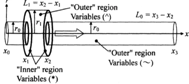
This paper considersasimple axisymmetric‘silencer model’ consistingofanexpansion
cham-berfollowed by a tailpipe, as shown in Fig. 1.
Figure 1: The expansion chamber-tailpipe system. Sketch of the configuration of the problem,
and indication of coordinates.
The aim is to contribute to the understandingof the interaction betweenoscillations of the
flow field and the acoustic field. By oscillations of the flow field
we mean
the self-sustainedoscillations ofthe jet shearlayer. Theshearlayer is unstable and rolls upinto alarge, coherent
vortex ($a$ ‘smoke-ring’) which is convected downstream with the flow. It cannot pass through
disturbance is thrown back (with the speed
of
sound) to the upstream plate, where it disturbsthe shear layer. This initiates the roll-up of
a new
coherent vortex. In this wayan
acousticfeedback loop is formed, making up
one
type offlow-acoustic interaction.These so-called hole-tone feedback oscillations [2, 14, 15, 22] may interact with the acoustic
axial and (to a much lesser extend) radial eigen-oscillations in the cavity and in the tailpipe
[3, 6]. In the present paper
we
seek to understand the interaction with the axialwaves
in thetailpipe.
As indicated in Fig. 1, perfect axisymmetry is assumed, and a mathematical model is
formulated in terms of the cylindrical axisymmetric coordinates $(x, r)$
.
The sound-generatingflowis represented by
a
discrete vortex method approach, based on (axisymmetric) vortex rings,as
applied also in earlier papers [14, 15]. The acoustic part of the problemcan
be solvedanalytically, andcompletely, interms of eigenfunction expansions.
A
travellingwave
formulationfor
a
single change in cross-sectionalarea
was
considered already in1944
by Miles [19]. TheresultsofMiles
were
employed by El-Sharkawy&
Nayfeh [5] inananalysisof sound propagationthrough
an
expansion chamber. The problem of Mileswas
reconsidered by Dup\‘ere&
Dowling[4] in terms of Howe’s theoryofvortex sound [8, 9].
$A$ ‘brute-force’ eigenfunction expansion solution,
as
mentioned above, will actually becomequite complicated. A much
more
manageable approach is possible by taking advantage ofcharacteristic length-scales in the different regions of the problem: (i) tailpipe region, (ii) step
(cross section change) regions, and (iii) cavity region. The simplified solutions for these three
regions canthen be coupled by employing the method of matched asymptotic expansions. Such
an approach
was
usedby Lesser&
Lewis [16, 17] for a plane (two-dimensional) duct. It is alsothe approach employed in the present paper.
The paper is divided into eight sections. The (time-domain) governing equations
are
givenand discussed in Section 2. The brief
Section
3
is concerned with Fourier transform, used inorder to go from
a
time-domain toa
frequency-domain formulation. Section 4 is concernedwith non-dimensionalization in terms ofparameters with appropriate length- and time-scales.
A perturbationexpansion ofthe dependent variables is discussed in Section 5. This is followed
by solutions of the simplified governing equations. Asymptotic matching of these solutions
is discussed in Section 6. Transformation back to the time-domain is discussed in Section 7.
Finally, concluding remarks
are
madein Section 8.2
Governing
equations
The starting point is taken in the Euler equation [8]
$\rho\frac{\partial u}{\partial t}+\nabla p=-\rho \mathfrak{L}H(x-x_{1})H(x_{2}-x)$, (1)
where$\rho$is themeandensity of thefluid, $t$is thetime, $u=(u, v)$ is the acoustic particle velocity,
$p$ is the acoustic pressure, and
$\mathfrak{L}=\omega\cross v$, (2)
which often is called the vortex force,
or
the Lamb vector [8, 9]. In this expression, $v=(u, \mathfrak{v})$isflowvelocityofthe incompressible, sound-generating ‘backgroundflow’ and$\omega=\nabla\cross v$ isthe
vorticity. Finally, $H(s)$ is the Heavisidestep function, which equals$0$ for $s<0$ and 1 for $s>0.$
The continuity equation is
$\kappa\frac{\partial p}{\partial t} = -\nabla\cdot u$ (3) $= -[ \frac{\partial u}{\partial x}+\frac{1}{r}\frac{\partial}{\partial r}(rv)],\kappa=\frac{1}{\rho c_{0}^{2}},$
where $c_{0}$ is the speed of sound.
Equations(1)and (3)canbe combinedthroughelimination of$u$togivethe non-homogeneous
waveequation
$\frac{1}{k}\frac{\partial p}{\partial t^{2}}-\nabla^{2}p=\rho\nabla\cdot \mathfrak{L}H(x-x_{1})H(x_{2}-x)$
.
(4)Equation (1) shouldbe understood in the sameway as the Powell-Howe equation (4) normally
isunderstood [8, 9], thatis, it is assumed thattheobservationpoint $(x, r)$ is well away from the
sound source domain, such that the fluid dynamical flow velocity $v\approx O$ there (giving also that
$\mathfrak{L}\approx 0)$
.
In terms ofa flow (shear layer) representation by a ‘necklace’ of $M$ discrete axisymmetric
vortexrings, located at $(x_{m}, r_{m})$, $m=1$,2,$\cdots,$$M$, the Lamb vector $\mathfrak{L}=(\mathfrak{L}_{x}, \mathfrak{L}_{r})$ is given by
$\mathfrak{L}=(\mathfrak{L}_{x}, \mathfrak{L}_{r})=\sum_{m=1}^{M}\Gamma_{m}\delta(x-x_{m})\frac{\delta(r-r_{7n})}{\pi r}(0_{m}, -u_{m})$
.
(5)Here $\delta(x-x_{m})$ is the one-dimensional delta function ([10], p. 55), while $\delta(r-r_{m})/\pi r$ is the
axisymmetric deltafunction ([10], p. 306).
3
Fourier
transform
Solution of the equations, and asymptotic matching of these solutions, is easier to carry out in
the frequency domain, rather than in the time domain. We thus employ the Fourier transform
$P( \omega)=\int_{-\infty}^{\infty}p(t)e^{i\omega t}dt, p(t)=\frac{1}{2\pi}\int_{-\infty}^{\infty}P(\omega)e^{-i\omega t}d\omega$, (6)
to obtain the frequency domain Euler equation
$i\rho\omega U=\nabla P+\rho LH(x-x_{1})H(x_{2}-x)$, (7)
and the continuity equation
$i\omega\kappa P=\nabla\cdot$ U. (8)
The frequencydomain version of(4) takes the form
$\nabla^{2}P+k^{2}P=-\rho\nabla\cdot LH(x-x_{1})H(x_{2}-x)$, (9)
where $k=\omega/c_{0}$ is the acoustic
wave
number. ThetransformedLamb vector $L=\Omega\cross V$, where$\Omega=\nabla\cross V.$
4
Scaling
The governing equations (7), (8), and (9)
are
made non-dimensional by theuse
ofappropriatelength scales for each of the three types of domain, (i) pipe domain, (ii) step domain, and (iii)
cavity domain. In the following, let $U=(U, V)$ and let $V=(U, \mathfrak{B})$
.
(i) Pipe domain. Here the pipe length$L_{0}$ is the appropriate length scale in the$x$direction, while
the piperadius $r_{0}$ is appropriate inthe $r$direction. We thus get
$\tilde{x}=\frac{x}{L_{0}}, \tilde{r}=\frac{r}{r_{0}}, \tilde{u}=\frac{U}{\omega L_{0}}, \tilde{v}=\frac{V}{\omega r_{0}}, \tilde{p}=\frac{P}{\rho c_{0}\omega L_{0}}, \tilde{k}=kL_{0}$
.
(10)(ii) Step domain. Here the geometry is rapidly varying, and
we
thus make both $x$ and $r$slowly
across
thestep, and $\omega L_{0}$ is the appropriatevelocityscale in both$x$ and$r$ directions. Wethus get
$x^{*}= \frac{x}{r_{0}}=\frac{\tilde{x}}{\epsilon}, r^{*}=\frac{r}{r_{0}}, u^{*}=\frac{U}{\omega L_{0}}, v^{*}=\frac{V}{\omega L_{0}}=\tilde{v}\epsilon$, (11)
$p^{*}= \frac{P}{\rho c_{0}\omega L_{0}}, k^{*}=kL_{0}.$
(iii) Cavity domain. Here
we
willassume
that the long length-scale$L_{0}$ isthe appropriateone
inboth $x$ and $r$directions. We thus get
$\hat{x}=\frac{x}{L_{0}}, \hat{r}=\frac{r}{L_{0}}=\tilde{r}\epsilon, \hat{u}=\frac{U}{\omega L_{0}}=\frac{\tilde{u}}{\epsilon}, \hat{v}=\frac{V}{\omega L_{0}}, \hat{p}=\frac{P}{\rho c_{0}\omega L_{0}}$, (12)
$\hat{k}=kL_{0}, \hat{L}=\frac{L}{\rho c_{0}\omega}, \hat{\Gamma}_{m}=\frac{\Gamma_{m}}{\rho c_{0}L_{0}^{2}}, \hat{u}=\frac{\mu}{\omega L_{0}}, \hat{\mathfrak{v}}=\frac{\mathfrak{B}}{\omega L_{0}}.$
4.1
Scaled governing equations
Using the non-dimensionalparametersintroduced in the previous Section,
we
obtainthefollow-ing scaled, non-dimensionalequations.
(i) Pipe domain
$ik\tilde{u}=\frac{\partial\tilde{p}}{\partial\tilde{x}}, \epsilon^{2}i\tilde{k}=\frac{\partial\tilde{p}}{\partial\tilde{r}}, i\tilde{k}\tilde{p}=\frac{\partial\tilde{u}}{\partial\tilde{x}}+\frac{\tilde{v}}{\tilde{r}}+\frac{\partial\tilde{v}}{\partial\tilde{r}}$
.
(13)(ii) Step domain
$\epsilon ik^{*}u^{*}=\frac{\partial p^{*}}{\partial x^{*}}, \epsilon ik^{*}v^{*}=\frac{\partial p^{*}}{\partial r^{*}}, \epsilon ip^{*}=\frac{\partial u^{*}}{\partial x^{*}}+\frac{v^{*}}{r}*+\frac{\partial v^{*}}{\partial r^{*}}$
.
(14)(iii) Cavity domain
$i\hat{k}\hat{u}=\frac{\partial\hat{p}}{\partial\hat{x}}+\hat{L}_{x}, i\hat{k}\hat{v}=\frac{\partial\hat{p}}{\partial\hat{r}}+\hat{L}_{r}, i\hat{k}\hat{p}=\frac{\partial\hat{u}}{\partial\hat{x}}+\frac{\hat{v}}{\hat{r}}+\frac{\partial\hat{v}}{\partial\hat{r}}$, (15)
$\frac{\partial^{2}\hat{p}}{\partial\hat{x}^{2}}+\frac{1}{\hat{r}}\frac{\partial\hat{p}}{\partial\hat{r}}+\frac{\partial^{2}\hat{p}}{\partial\hat{r}^{2}}+\hat{k}^{2}\hat{p} = -\hat{\nabla}\cdot\hat{L}$,
(16) $= - \frac{\partial\hat{L}_{x}}{\partial\hat{x}}-\frac{1}{\hat{r}}\frac{\partial}{\partial\hat{r}}(\hat{r}\hat{L}_{r})$
.
In all of these equations, $\epsilon=r_{0}/L_{0}$ play the role of
a
small parameter.5
Perturbation expansion, simplified
equations,
and solutions
Next the dependent variables$p,$ $u$, and $v$ (with
a
tilde,a
hat,or
an
asterisk)are
expanded interms ofasymptotic sequences of functions of$\epsilon$ (defined$ju_{\iota}st$ above),
$p = \alpha_{0}(\epsilon)p_{0}+\alpha_{1}(\epsilon)p_{1}+\alpha_{2}(\epsilon)p_{2}+\cdots$ , (17)
$u = \beta_{0}(\epsilon)u_{0}+\beta_{1}(\epsilon)u_{1}+\beta_{2}(\epsilon)u_{2}+\cdots,$
$v = \gamma_{0}(\epsilon)v_{0}+\gamma_{1}(\epsilon)v_{1}+\gamma_{2}(\epsilon)v_{2}+\cdots$
In the most general approach, $\alpha_{n}(\epsilon)$, $\beta_{n}(\epsilon)$, and $\gamma_{n}(\epsilon)$
are
asymptotic sequences of unknowncase it is, however, sufficient to let these functions be simple powers of $\epsilon$
.
Thus we apply theexpansions
$p = p_{0}+\epsilon p_{1}+\epsilon^{2}p_{2}+\cdots$ , (18) $u = u_{0}+\epsilon u_{1}+\epsilon^{2}u_{2}+\cdots,$
$v = v_{0}+\epsilon v_{1}+\epsilon^{2}v_{2}+\cdots$
To the lowest $(\epsilon^{0})$ order,
the governing equations in the pipe section
are
$i\tilde{k}\tilde{u}_{0}=\frac{\partial\tilde{p}_{0}}{\partial\tilde{x}}, \frac{\partial\tilde{p}_{0}}{\partial\tilde{r}}=0$
, (19)
$i\tilde{k}\tilde{p}_{0}=\frac{\partial\tilde{u}_{0}}{\partial\tilde{x}}+\frac{\tilde{v}_{0}}{\tilde{r}}+\frac{\partial\tilde{v}_{0}}{\partial\tilde{r}}.$
The second equationof(19) gives that$\tilde{p}_{0}$ isa function of$x$ only, i.e. $\tilde{p}_{0}(x)$
.
Usingthis, one findsthat the acoustic particle velocity components aregoverned by the equations
$\tilde{u}_{0}=\frac{1}{i\tilde{k}}\frac{\partial\tilde{p}_{0}}{\partial\tilde{x}}, \tilde{v}_{0}=-\frac{\tilde{r}}{i2\tilde{k}}[\frac{\partial^{2}\tilde{p}_{0}}{\partial\tilde{x}^{2}}+\tilde{k}^{2}\tilde{p}_{0}]$
.
(20)
Applying the second of these equations on the pipe wall $\tilde{r}=\tilde{r}_{0}$ (where $\tilde{v}_{0}=0$), one finds that
thepressure$\tilde{p}_{0}$ is governed by the one-dimensional
wave
equation contained within the squarebrackets $[]$ in (20). The solutiontothisequation, whichsatisfies the boundary condition
$\tilde{p}_{0}=0$
at $\tilde{x}=\tilde{x}_{3}$, is given by
$\tilde{p}_{0}=\tilde{p}_{0}(\tilde{x})=A_{0}[\cos\tilde{k}\tilde{x}-\cot\tilde{k}\tilde{x}_{3}\sin\tilde{k}\tilde{x}]$ . (21)
The step sections are, to the lowest order, governed by
$\frac{\partial p_{0}^{*}}{\partial x^{*}}=0, \frac{\partial p_{0}^{*}}{\partial r^{*}}=0$,
(22)
$ik^{*}u_{0}^{*}=\frac{\partial p_{1}^{*}}{\partial x^{*}}, ik^{*}v_{0}^{*}=\frac{\partial p_{1}^{*}}{\partial r^{*}}.$
The first two equations give that
$p_{0}^{*}=C_{0}^{*}=$ constant. (23)
As the next two equations show, the lowest order velocity components
are
governed by thenext-order $(\epsilon^{1})$ pressure term, $p_{1}^{*}$
.
Thisterm is governed by the Laplace equation$\frac{\partial^{2}p_{1}^{*}}{\partial x^{*2}}+\frac{1}{r^{*}}\frac{\partial p_{1}^{*}}{\partial r^{*}}+\frac{\partial^{2}p_{1}^{*}}{\partial r^{*2}}=0$
.
(24)
Concentrating here on the step at $x^{*}=x_{2}^{*}$ (refer to Fig. 1), the solution to (24) there can be
written as
$p_{1}^{*}=\{\begin{array}{l}a_{0}^{*-}+\sum_{n}a_{n}^{*-}e^{-\zeta_{n}\epsilon x^{*}}1J_{0}(\zeta_{n}\epsilon_{1}r^{*}) , x^{*}<x_{2}^{*},a_{0}^{*+}+\sum_{n}a_{n}^{*+}e^{-\zeta_{n}x^{*}}J_{0}(\zeta_{n}r^{*}) , x^{*}>x_{2}^{*},\end{array}$ (25)
where$J_{0}$ is the Bessel function of first kind and order zero.
On the step at $x^{*}=x_{2}^{*}$, the following boundary conditions must be satisfied:
$p_{1}^{*}(x_{2}^{*-}, r^{*}) = p_{1}^{*}(x_{2}^{*+}, r^{*}) , 0<r^{*}<1$, (26)
$\frac{\partial p_{1}^{*}}{\partial x^{*}}(x_{2}^{*-},r^{*}) = \frac{\partial p_{1}^{*}}{\partial x^{*}}(x_{2}^{*+}, r^{*}) , 0<r^{*}<1,$
where$\epsilon_{1}=r_{0}/r_{1}$ (see again Fig. 1). As it isnot possible to imposethese ‘strong conditions’
on
asolution of the form (25), will will instead employ the following equivalent weak conditions,
$\int_{0}^{1}p_{1}^{*}(x_{2}^{*-}, r^{*})J_{0}(\zeta_{m}r^{*})r^{*}dr^{*} = \int_{0}^{1}pi(x_{2}^{*+}, r^{*})J_{0}(\zeta_{m}r^{*})r^{*}dr^{*}$, (27) $\int_{0}^{1}\frac{\partial p_{1}^{*}}{\partial x^{*}}(x_{2}^{*-}, r^{*})r^{*}dr^{*} = \int_{0}^{1}\frac{\partial p_{1}^{*}}{\partial x^{*}}(x_{2}^{*+}, r^{*})r^{*}dr^{*},$
$\int_{1}^{1/\epsilon_{1}}\frac{\partial p_{1}^{*}}{\partial x^{*}}(x_{2}^{*-},r^{*})r^{*}dr^{*}$ $=$ O.
It is noted that the last two conditions
can
be combined into one,on
the form$\int_{0}^{1/\epsilon_{1}}\frac{\partial p_{1}^{*}}{\partial x^{*}}(x_{2}^{*-},r^{*})r^{*}dr^{*}=\int_{0}^{1}\frac{\partial p_{1}^{*}}{\partial x^{*}}(x_{2}^{*+}, r^{*})r^{*}dr^{*}$
.
(28)The applicationofthese boundaryconditions willbe discussedin connectionwith the matching
of solutions in the next Section.
For the expansion chamber, it isconvenient tostatethe lowest $(\epsilon^{0})$ ordergoverning equation
on the
wave
equationform$\frac{\partial^{2}\hat{p}_{0}}{\partial\hat{x}^{2}}+\frac{1}{\hat{r}}\frac{\partial\hat{p}_{0}}{\partial\hat{r}}+\frac{\partial^{2}\hat{p}_{0}}{\partial\hat{r}^{2}}+\hat{k}^{2}\hat{p}_{0}=-\hat{\nabla}$
.
$\hat{L}$.
(29)A particular solution
can
be expressedas
$\hat{p}_{0}^{part}=\iint G\nabla\cdot\hat{L}\hat{r}d\hat{r}d\hat{x}=-\iint\hat{L}\cdot(\frac{\partial G}{\partial\hat{x}}, \frac{\partial G}{\partial\hat{r}})\hat{r}d\hat{r}d\hat{x}$, (30)
where the superscript ‘part’ refersto ‘particular’, and
$G(x, r)= \frac{i}{2\pi\hat{\delta}^{2}}\sum_{n=0}^{\infty}\frac{1}{\kappa_{n}}\frac{J_{0}(\zeta_{n}\hat{r}_{*}/\hat{\delta})}{J_{0}^{2}(\zeta_{n})}J_{0}(\zeta_{n}\frac{\hat{r}}{\hat{\delta}})e^{i\kappa_{n}|\hat{x}-\hat{x}.|}$ (31)
is the Green’s function which satisfies the boundary condition $\partial G/\partial\hat{r}=0$ at $\hat{r}=\hat{r}_{1}$
.
Here$\kappa_{n}=\{\begin{array}{l}\sqrt{\hat{k}^{2}-(\zeta_{n}/\hat{\delta})^{2}} for |\hat{k}|>\zeta_{n}/\hat{\delta}i\sqrt{(\zeta_{n}/\hat{\delta})^{2}-\hat{k}^{2}} for |\hat{k}|.<\zeta_{n}/\hat{\delta}\end{array}$
and $\zeta_{n}$
are
thethezeros
of$J_{1}$, the Bessel function oforder unity. For convenience,we
willwrite (30) as$\hat{p}_{0}^{part}=\sum_{m=1}^{M}\sum_{n=0}^{\infty}\hat{f}_{n}(\hat{r},\hat{r}_{m})e^{i\kappa_{n}|\hat{x}-\hat{x}_{m}|}$, (32)
where $(\hat{x}_{m},\hat{r}_{m})$ are, again, the positionsofthe freevortex rings present within the cavity, and
$\hat{f}_{n}(\hat{r},\hat{r}_{m})=-\frac{\hat{\Gamma}_{m}}{2\pi\hat{\delta}^{2}}\frac{J_{0}(\zeta_{n}\frac{\hat{r}}{\delta})}{J_{0}^{2}(\zeta_{n})}[\hat{\mathfrak{v}}_{m}J_{0}(\zeta_{n}\frac{\hat{r}_{m}}{\hat{\delta}})+i\hat{u}_{m}\frac{\zeta_{n}}{\kappa_{n}\hat{\delta}}J_{1}(\zeta_{n}\frac{\hat{r}_{m}}{\hat{\delta}})]$
.
(33)Wewillalsoinclude an‘eigensolution’ to the homogeneous versionof(29), which likewise satisfies
the boundary condition$\partial G/\partial\hat{r}=0$ at $\hat{r}=\hat{r}_{1}$. Such
a
solutioncan
bewrittenas
wherethe superscript ‘hom’ refers to (homogeneous’. The full (complete) solution is thus
$\hat{p}_{0}=\hat{p}_{0}^{part}+\hat{p}_{0}^{h\circ m}$
.
(35)
Evaluation of the acoustic particle velocity components will be based on the ‘homogeneous
solution’ (34) only,
$i\hat{k}\hat{u}_{0}=\frac{\partial\hat{p}_{0}^{hom}}{\partial\hat{x}}, i\hat{k}\hat{v}_{0}=\frac{\partial\hat{p}_{0}^{hom}}{\partial\hat{r}}$
.
(36)6
Asymptotic matching of solutions
We first match the solutions (21) and (23), for the pipe and step regions, respectively. Here
$p_{0}(x)$ (for the pipe) is considered
as
the outerexpansion and$p_{0}^{*}(x^{*})$ (for the step)
as
the innerexpansion. The outer variable is $\tilde{x}=x/L_{0}$, while the inner variable is $x^{*}=(x-x_{2})/r_{0}=$
$(\tilde{x}-\tilde{x}_{2})/\epsilon$, which gives that$\tilde{x}=\epsilon x^{*}+\tilde{x}_{2}$
.
The matchingprinciple applied here is ([21], p.266)
Inner expansion of(outer expansion) $=$ Outerexpansion of (inner expansion), (37)
which for thepresent pipe-step matching problem takesthe form
$\lim_{\epsilonarrow 0} p_{0}^{*}(\frac{\tilde{x}-\tilde{x}_{2}}{\epsilon})= \lim_{\epsilonarrow 0} \tilde{p}_{0}(\epsilon x^{*}+\tilde{x}_{2})$. (38)
$\tilde{x}-\tilde{x}_{2}$ fixed $x^{*}$ fixed
Evaluation of (38) gives the relation
$C_{0}^{*}=\tilde{A}_{0}\{\cos\tilde{k}\tilde{x}_{2}-\cot\tilde{k}\tilde{x}_{3}\sin\tilde{k}\tilde{x}_{2}\}$
.
(39)Next we will match (23) for the (downstream) step with (32) for the cavity. That is to
say, in the cavity, only the particular solution$\hat{p}_{0}^{part}$
will be considered. (The homogeneous part
of the cavity-solution, $\hat{p}_{0}^{hom}$, will be determined in connection with matching of axial velocity
components;
see
a little later.) The outer variable is now $\hat{x}=\tilde{x}=x/L_{0}$. The inner variable is $x^{*}=(x-x_{2})/r_{0}=(\hat{x}-\hat{x}_{2})/\epsilon$, giving$\hat{x}=\epsilon x^{*}+\hat{x}_{2}$.
A limiting process similar to (38) nowgives $C_{0}^{*}= \sum_{\gamma n}\sum_{n}\hat{f}_{n}(\hat{r},\hat{r}_{m})e^{i\kappa_{n}|\hat{x}_{2}-\hat{x}_{m}|}$.
(40)As (23) prescribes, $C_{0}$ is to be a constant. We thus take the
mean
valueover $\hat{r},$
$\int_{0}^{\hat{\delta}}C_{0}^{*}d\hat{r}=\sum_{m}\sum_{n}\int_{0}^{\hat{\delta}}\hat{f}_{n}(\hat{r}_{)}\hat{r}_{m})e^{i\kappa_{n}|\hat{x}_{2}-\hat{x}_{m}|}d\hat{r} \Rightarrow$
(41)
$C_{0}^{*}= \sum_{m}\sum_{n}\frac{1}{\hat{\delta}}\int_{0}^{\hat{\delta}}\hat{f}_{n}(\hat{r},\hat{r}_{m})e^{i\kappa_{n}|\hat{x}_{2}-\hat{x}_{m}|}d\hat{r}.$
In this way we obtain the pressure within the pipeon the form
$\tilde{p}_{0}=\sum_{m=1}^{M}\sum_{n=0}^{\infty}\frac{1}{\hat{\delta}}\int_{0}^{\hat{\delta}}\hat{f}_{n}(\hat{r},\hat{r}_{m})d\hat{r}e^{i\kappa_{n}|\hat{x}_{2}-\hat{x}_{m}|}\frac{\sin\tilde{k}(\tilde{x}_{3}-\tilde{x})}{\sin\tilde{k}(\tilde{x}_{3}-\tilde{x}_{2})}$
.
(42)As to the averaging
over
$\hat{r}$, it is noted that averaging overthe cross-sectional area, on theform
$\hat{\delta}$
$\int_{0}\cdots\hat{r}d\hat{r}$, probably is more natural; this integral is however equal to
zero.
Evaluationofthe
averaging integral in (41), (42) gives
$\frac{1}{\hat{\delta}}\int_{0}^{\hat{\delta}}\hat{f}_{n}(\hat{r},\hat{r}_{m})d\hat{r}=-\frac{\hat{\Gamma}_{m}}{2\pi\hat{\delta}^{2}}\frac{1-\frac{\pi}{2}H_{1}(\zeta_{n})}{J_{0}(\zeta_{n})}[\hat{\mathfrak{v}}_{m}J_{0}(\zeta_{n}\frac{\hat{r}_{m}}{\hat{\delta}})+i\hat{u}_{\mathfrak{m}}\frac{\zeta_{n}}{\kappa_{n}\hat{\delta}}J_{1}(\zeta_{n}\frac{\hat{r}_{m}}{\hat{\delta}})]$
where$H_{1}$ is the Struve function of order unity ([1], p. 496).
It is interesting to note that (42) hasaformsimilarto the
case
where thepressurepulsationsin the pipe are driven by
an
oscillating pistonat $\tilde{x}=\tilde{x}_{2}$ ([13], p. 176). The$P_{\sim}^{ressure}$ amplitude
will go to infinity at the pipe
resonance
frequencies $\tilde{k}\tilde{\ell}=j\pi,$ $j=1$, 2,$\cdots$, where $\ell=\tilde{x}_{3}-\tilde{x}_{2}$is the length of the pipe. Contrary to
resonance
in (solid) mechanical oscillators with viscousdamping, this (ca.seofinfiniteamplitude)remainstrue
even
whenviscosity isincluded (seeagain[13], p. 176).
Next we will consider matching of the axial velocity components. For the pipe section we
have$\partial\tilde{p}_{0}/\partial\tilde{x}=i\tilde{k}\tilde{u}_{0}$, giving
$\tilde{u}_{0}=i\tilde{A}_{0}\{\sin\tilde{k}\tilde{x}+\cot\tilde{k}\tilde{x}_{3}\cos\tilde{k}\tilde{x}\}$
.
(44)For the step
we
have $\partial pi/\partial x^{*}=ik^{*}u_{0}^{*}$, giving (just downstream of the step)$u_{0}^{*}=Y_{0}^{*+}a_{0}^{*+}+ \sum_{n=1}^{\infty}Y_{n}^{*+}a_{n}^{*+}e^{-\lambda_{n}x^{*+}}J_{0}(\lambda_{n}r^{*})$, (45)
wherethecoeffcients$Y_{n}^{*+}$, andlikewise$Y_{n}^{*-}$just upstreamofthe step,
are
acoustic admittances([11], [18], p. 104), definedby
$Y_{n}^{*\pm}= \frac{1}{ik^{*}p_{1n}^{*\pm}}\frac{\partial p_{1n}^{*\pm}}{\partial x^{*\pm}}$
.
(46)Here$p_{1n}^{*\pm}$ is the n’th term in the expansion (25).
Now
$\lim_{\epsilonarrow 0} u_{0}^{*}(\frac{\tilde{x}-\tilde{x}_{2}}{\epsilon})= \lim_{\epsilonarrow 0} \tilde{u}_{0}(\epsilon x^{*}+\tilde{x}_{2})$ (47)
$\tilde{x}-\tilde{x}_{2}$ fixed $x^{*}$ fixed
gives
$Y_{0}^{*+}a_{0}^{*+}=i\tilde{A}_{0}\{\sin\tilde{k}\tilde{x}_{2}+\cot\tilde{k}\tilde{x}_{3}\cos\tilde{k}\tilde{x}_{2}\}$
.
(48)Next, for the cavity
we use
$\partial\hat{p}_{0}^{hom}/\partial\hat{x}=i\hat{k}\hat{u}_{0}$.
Matching then gives$Y_{0}^{*-}a_{0}^{*-}= \sum_{n=0}^{\infty}i\kappa_{n}J_{0}(\zeta_{n}\frac{\hat{r}}{\hat{\delta}})\hat{C}_{n}e^{i\kappa_{\mathfrak{n}}\hat{x}_{2}}$, (49)
where (28) gives that $Y_{0}^{*+}$ is related to$Y_{0}^{*-}$
as
follows:$Y_{0}^{*-}a_{0}^{*-}=\epsilon_{1}^{2}Y_{0}^{*+}a_{0}^{*+}$, (50)
where, again, $\epsilon_{1}=r_{0}/r_{1}.$
In order to determine the coefficients $\hat{C}_{n}$
, we multiply both sides of (49) by $J0(\zeta_{m}^{\hat{r}}\delta)\hat{r}/\hat{\delta},$
and integrateover $\hat{r},$
$Y_{0}^{*-}a_{0}^{*-} \int_{0}^{1}J_{0}(\zeta_{m}\frac{\hat{r}}{\hat{\delta}})\frac{\hat{r}}{\hat{\delta}}d\frac{\hat{r}}{\hat{\delta}}=\sum_{n=0}^{\infty}i\kappa_{n}\hat{C}_{n}e^{i\kappa_{\mathfrak{n}}\hat{x}2}\int_{0}^{1}J_{0}(\zeta_{m}\frac{\hat{r}}{\hat{\delta}})J_{0}(\zeta_{n}\frac{\hat{r}}{\hat{\delta}})\frac{\hat{r}}{\hat{\delta}}d\frac{\hat{r}}{\hat{\delta}}$
.
(51)This gives
$i\kappa_{0}\hat{C}_{0}=Y_{0}^{*-}a_{0}^{*-}$ (52)
Thus
we
obtain the axial feedbackvelocity component within the cavityon the form$\hat{u}_{0}=\epsilon_{1}^{2}\frac{e^{i\kappa_{n}|\hat{x}-\hat{x}_{2}|}}{\hat{k}}\cot\tilde{k}(\tilde{x}_{3}-\tilde{x}_{2})\sum_{m=1}^{M}\sum_{n=0}^{\infty}\frac{1}{\hat{\delta}}\int_{0}^{\hat{\delta}}\hat{f}_{n}(\hat{r},\hat{r}_{m})d\hat{r}e^{i\kappa_{\mathfrak{n}}|\hat{x}-\hat{x}_{n}|}2$
.
(53)As bythe pressure equation (42), the velocityamplitudewill goto infinityat thepipe
resonance
frequencies $\tilde{k}\tilde{\ell}=j\pi,$
$j=1$, 2,$\cdots,$
7
Time domain expressions
Finally, the mostimportant frequency-domainexpressions (42) and (53) (with (43)) arereverted
to thetime domainby employingthe second ofthe equations (6). It
seems
to be most convenienttoinvert certain blocks one at a time (see the Appendix), andthen couple these blocks via the
convolutiontheorem([20], p. 464). Thefinal expression for the pressure within the tailpipe (42)
is
$\tilde{p}_{0}(\tilde{x},\tau)=\hat{\delta}^{-2}\sum_{j=1}^{\infty}\sum_{m=1}^{M}\sum_{n=0}^{\infty}\int_{0}^{\tau}\int_{0}^{\tau}\frac{\Gamma_{m}(\alpha)}{J_{0}(\zeta_{n})}\{1-\frac{\pi}{2}H_{1}(\zeta_{n})\}\cross$ (54)
$\cross(-1)^{j+1}\tilde{\ell}^{-1}\sin\frac{j\pi}{\tilde{\ell}}(\tilde{x}_{3}-\tilde{x})\sin\frac{j\pi}{\tilde{\ell}}(\tau-\alpha-\beta)x$
$\cross[\hat{\mathfrak{v}}_{m}(\alpha)J_{0}(\zeta_{n}\frac{\hat{r}_{m}}{\hat{\delta}})\frac{\partial}{\partial\hat{x}_{2}}H_{0}^{(1)}(T_{mn}(\beta))-\hat{\iota}\downarrow_{m}(\alpha)J_{1}(\zeta_{n}\frac{\hat{r}_{m}}{\hat{\delta}})H_{0}^{(1)}(T_{mn}(\beta))]d\alpha d\beta,$
where$\tilde{\ell}=\tilde{x}_{3}-\tilde{x}_{2}$
is the length of the tailpipe, and
$T_{mn}(\tau)=\{\begin{array}{ll}\ \sqrt{\tau^{2}-|\hat{x}_{2}-\hat{x}_{m}|^{2}} for \tau^{2}>|\hat{x}_{2}-\hat{x}_{m}|^{2}i_{\delta}g_{\sqrt{|\hat{x}_{2}-\hat{x}_{m}|^{2}-\tau^{2}}} for \tau^{2}<|\hat{x}_{2}-\hat{x}_{m}|^{2}\end{array}$
(55)
The final expression for the axialfeedback velocity component within the cavity (53) is
$\hat{u}_{0}(\hat{x}, \tau)=-\frac{\epsilon_{1}^{2}}{\hat{\delta}^{2}}\sum_{j=1}^{\infty}\sum_{m=1}^{M}\sum_{n=0}^{\infty}\int_{0}^{\tau}\int_{0}^{\tau}\int_{0}^{\tau}\frac{\Gamma_{m}(\alpha)}{J_{0}(\zeta_{n})}\{1-\frac{\pi}{2}H_{1}(\zeta_{n})\}\cross$ (56)
$\cross[\hat{\mathfrak{v}}_{m}(\alpha)J_{0}(\zeta_{n}\frac{\hat{r}_{m}}{\hat{\delta}})\frac{\partial}{\partial\hat{x}_{2}}H_{0}^{(1)}(T_{mn}(\beta))-\hat{u}_{m}(\alpha)J_{1}(\zeta_{n}\frac{\hat{r}_{rn}}{\hat{\delta}})H_{0}^{(1)}(T_{mn}(\beta))]\cross$
$\cross\tilde{\ell}^{-1}\sin\frac{j\pi}{\tilde{\ell}}(\tau-\alpha-\beta-\gamma)H(\gamma-|\hat{x}_{2}-\hat{x}|)d\alpha d\beta d\gamma.$
8
Concluding
remarks
1. Analytical (approximate) expressions have beenobtained, via matched asymptotic
expan-sions, for the pressure and the axial component of the acoustic feedback velocity in a
cavity-pipe system.
2. The radial component of the acoustic feedback velocity does not
come
into play by theorder of analysis considered here. It is intuitively understandable that
a
radial velocitycomponent borne from the purely axial pipe oscillations necessarily must be very small.
Yet its effect might not be negligibly small, and it would be ofinterest to continue the
analysis to higher orders.
3. Just
as
by the pressure in the pipe, the amplitude of the axial component of the acousticfeedback velocity becomes infinite at the pipe
resonance
frequencies. This indicates thepossibility of lock-in of the self-sustained flow oscillations in the cavity to the resonant
acoustic pipe pressure oscillations.
4. Future workwill, first andforemost, be concerned with numerical computationsbased on
thepresentresults. Asto extensions of theanalyticalwork (besidesthe higher order terms
mentionedjust above) inclusion of the free space solution (downstream from the free pipe
end), along the lines discussed in the second of the two papers by Lesser
&
Lewis [17], would be interesting.Acknowledgement: The work reported here is being supported by a Collaborative Research
Appendix.
Fourier
inversions
In the inversionof(42), a useful result is that
$\frac{1}{2\pi}\int_{-\infty}^{\infty}\frac{\sin\tilde{k}(\tilde{x}_{3}-\tilde{x})}{\sin\tilde{k}\tilde{\ell}}e^{-i\overline{k}\tau}d\tilde{k}=\frac{1}{\pi\tilde{\ell}}\sum_{n=1}^{\infty}(-1)^{n+1}\sin\frac{n\pi}{\tilde{\ell}}(\tilde{x}_{3}-\tilde{x})\sin\frac{n\pi}{\tilde{\ell}}\tau$
.
(57)This result has been obtained by the method ofresidues. Similarly, for the inversion of (53),
use
is madeof that$\frac{1}{2\pi}\int_{-\infty}^{\infty}\cot\tilde{k}\tilde{\ell}e^{-i\overline{k}\tau}d\tilde{k}=-\frac{1}{\pi\tilde{\ell}}\sum_{n=1}^{\infty}\sin\frac{n\pi}{\tilde{\ell}}\tau$, (58)
and that
$\frac{1}{2\pi}\int_{-\infty}^{\infty}\frac{1}{i\kappa_{n}}e^{i\kappa_{n}|\hat{x}2^{-\hat{x}_{m}1}}e^{-i\overline{k}\tau}d\tilde{k}=-\frac{1}{2}H_{0}^{(1)}(T_{mn}(\tau))$, (59)
where$T_{mn}(\tau)$ is given by (55). $Rom(59)$
we can
obtain that$\frac{1}{2\pi}\int_{-\infty}^{\infty}e^{i\kappa_{\hslash}|\hat{x}2^{-\hat{x}_{n}1}}e^{-i\tilde{k}\tau}d\tilde{k}=-\frac{1}{2}\frac{\partial}{\partial\hat{x}_{2}}H_{0}^{(1)}(T_{mn}(\tau))$
.
(60)Finally, in (56) it has been usedalso that
$\frac{1}{2\pi}\int_{-\infty}^{\infty}\frac{1}{\hat{k}}e^{i\hat{k}|\hat{x}_{2}-\hat{x}_{m}|}e^{-i\hat{k}\tau}d\hat{k}=H(\tau-|\hat{x}_{2}-\hat{x}_{m}|)$, (61)
where $H$ is the Heavisideunit step function,
as
defined in connection with (1).References
[1] M. Abramowitz, I. A. Stegun, Handbook
of
Mathematical Frnctions, Dover Publications,New York,
1964.
[2] R. C. Chanaud, A. Powell, Someexperiments concerningthe hole and ringtone, J. Acoust.
Soc. Am. 37 (1965) 902-911.
[3] P. O. A. L. Davies, Flow-acousticcoupling in ducts, J. Sound Vibr. 77 (1981) 191-209.
[4] I. D. J. Dup\‘ere, A. P. Dowling, The absorption of sound
near
abrupt axisymmetricarea
expansions, J. Sound Vibr. 28 (2001)
709-730.
[5] A. I. El-Sharkawy, A. H. Nayfeh, Effect of an expansion chamber on the propagation of
sound in circular ducts, J. Acoust. Soc. Am. 63 (1978),
667-674.
[6] E. J. English, K. R. Holland, Aeroacousticsoundgeneration insimpleexpansionchambers,
J. Acoust. Soc. Am. 128 (2010),
2589-2595.
[7] H. Goyder, Noise generation and propagation within corrugated pipes, ASME J. Press.
Vessel Tech. 135 (2013),
130901
(1-7).[8] M. S. Howe, Acoustics
of
Fluid-Structure Interactions, Cambridge University Press,Cam-bridge, 1998.
[9] M. S. Howe, Theory
of
Vortex Sound, Cambridge UniversityPress, Cambridge, 2003.[10] D. S. Jones, The Theory
of
Generalised$\mathbb{R}$nctions, Cambridge University Press, Cambridge,[11] F. C. Karal, The analogous acoustical impedance for discontinuities and constrictions of
circular
cross
section, J. Acoust. Soc. Am. 25 (1953), 327-334.[12] J. Kevorkian, J. D. Cole, Perturbation Methods in Applied Mathematics, Springer-Verlag,
New York, 1981.
[13] H. Lamb, The Dynamical
Theow of
Sound, Dover Publications, New York, 2004 (orig. 1925).[14] M. A. Langthjem, M. Nakano, A numerical simulation of the hole-tone feedbackcyclebased
on anaxisymmetricdiscrete vortex method andCurle’sequation, J. Sound Vibr. 288(2005)
133-176.
[15] M. A. Langthjem, M. Nakano, Numerical study of the hole-tone feedback cycle based on
an
axisymmetric formulation. Fluid Dyn. Res. 42(2010) $015008(1-26)$.
[16] M.B. Lesser, J. A.Lewis, Applications ofmatched asymptotic expansion methods to
acous-tics. I. The Webster horn equation and the stepped duct, J. Acoust. Soc. Am. 51 (1972),
1664-1669.
[17] M. B. Lesser, J. A. Lewis, Applications of matched asymptoticexpansionmethods to
acous-tics. II. The open-ended duct, J. Acoust. Soc. Am. 52 (1972),
1406-1410.
[18] J. Lighthill, Waves in Fluids, Cambridge University Press, Cambridge, 1978.
[19] J. Miles, The reflection of sound due to a change in cross section of a circular tube, J.
Acoust. Soc. Am. 16 (1944), 14-19.
[20] P. M. Morse, H. Feshbach, Methods
of
Theoretical Physics I $\mathcal{E}i$II, Feshbach Publishing,
Minneapolis,
2004
(orig. 1953).[21] A. H. Nayfeh, introduction to Perturbation Methods, John Wiley
&
Sons, New York,1993.
[22] Lord Rayleigh, The Theory
of
Sound, Vol. II, DoverPublications, New York,1945.
[23] G. Rubio, W. De Roeck, J. Meyers, M. Baelmans, W. Desmet, Aeroacoustic noise source
mechanisms in simple expansion chambers. AIAA paper 2006-2700 (2006).
[24] A. Tamura, S. Takahashi, S. Sato, S. Hori, Numerical analysis ofsoundin the main steam