The second-order phase transition in the BCS-Bogoliubov model of superconductivity and its operator-theoretical proof (Mathematical Aspects of Quantum Fields and Related Topics)
11
0
0
全文
(2) 167 model without the magnetic fields is given by. (1.1). \Psi(T) = -2N_{0}\int_{\varepsilon}^{\hslash\omega_{D} \{\sqrt{\xi^{2}+u(T, \xi)^{2} -\xi\}d\xi. +N_{0} \int_{\varepsilon}^{\hslash\omega_{D} \frac{u(T,\xi)^{2} {\sqrt{\xi^{2}+ u(T,\xi)^{2} \tanh\frac{\sqrt{\xi^{2}+u(T,\xi)^{2} {2T}d\xi -4N_{0}T \int_{\varepsilon}^{\hslash\omega_{D} \ln\frac{1+e^{-\sqrt{\xi^{2}+ u(T,\xi)^{2} /T} {1+e^{-\xi/T} d\xi, T\in[\tau, T_{c}],. where N_{0}>0 and \omega_{D}>0 stand for the density of states per unit energy at the Fermi surface and for the Debye angular frequency, respectively. and u is the solution to the BCS‐Bogoliubov. gap equation (1.2) below. Here, \tau>0 is introduced in the next section, and T_{c}>0 is the transition temperature (see Definition 1.10 below) and satisfies \tau<T_{c} . We introduce \varepsilon>0, which is sufficiently small and fixed. We introduce a sufficientıy small. \varepsilon>0. because of some. mathematical reasons.. We consider the difference \Psi defined mainly on the closed interval [\tau, T_{c}] only. This is because we are interested in the phase transition at T=T_{c} and we need to study some properties of \Psi in the neighborhood of the transition temperature T_{c} . Definition 1.1. The transition to a superconducting state at the transition temperature T_{c} is a second‐order phase transition if the difference \Psi of the thermodynamic potential satisfies the following:. (a) \Psi\in C^{2}[\tau, T_{c}] and \Psi(T_{c})=0. (b) (c). \frac{\partial\Psi}{\partial T}(T_{c})=0.. \frac{\partial^{2}\Psi}{\partial T^{2} (T_{c})\neq 0.. Remark 1.2. Condition (a) of Definition 1.1 implies that the thermodynamic potential \Omega is continuous at an arbitrary temperature T . Conditions (a) and (b) imply that the entropy S=-(\partial\Omega/\partial T) is also continuous at an arbitrary temperature T and that, as a result, no latent heat is observed at T=T_{c} Hence conditions (a) and (b) imply the transition to a superconducting state at T_{c} is not a first‐order phase transition. On the other hand, Conditions. (a) and (c) imply that the specific heat at constant volume C_{V}=-T(\partial^{2}\Omega/\partial T^{2}) is discontinuous at T=T_{c} and that the gap \triangle C_{V} in C_{V} is observed at T=T_{c} . Here, the gap \triangle C_{V} at T=T_{c} is given by. \triangle C_{V}=-T_{c}\frac{\partial^{2}\Psi}{\partial T^{2} (T_{c}). .. For more detaiıs on the entropy and the specific heat at constant volume, see e.g. [2, Section III] or Niwa [11, Section 7.7.3]. In order to show that the transition to a superconducting state at the transition temperature. is a second‐order phase transition, we have to show that conditions (a), (b) and (c) of Definition 1.1 are all fulfilled. To this end, we need to differentiate the difference \Psi given by (1.1), and hence the solution. u. to the BCS‐Bogoliubov gap equation with respect to the temperature. T. two. times. We thus need to show that there is a unique (nonzero) solution to the BCS‐Bogoliubov gap equation and that the solution is differentiable with respect to the temperature two times..
(3) 168 The following is the welı‐known BCS‐Bogoliubov gap equation [2, 4] for superconductivity: (1.2). u(T, x)= \int_{\varepsilon}^{\hslash\omega_{D} \frac{U(x,\xi)u(T,\xi)} {\sqrt{\xi^{2}+u(T,\xi)^{2} \tanh\frac{\sqrt{\xi^{2}+u(T,\xi)^{2} {2T}d\xi,. T\geq 0,. \varepsilon\leq x\leq\hslash\omega_{D},. where the soıution u is a function of the absolute temperature T and the energy x . The potential U(\cdot, \cdot) satisfies U(x, \xi)>0 at aıl (x, \xi)\in[\varepsilon, \hslash\omega_{D}]^{2} . Here we again introduce \varepsilon>0 , which is sufficiently small and fixed. In the original BCS‐Bogoliubov gap equation, one sets \varepsilon=0. However we introduce a sufficiently smalı \varepsilon>0 because of some mathematical reasons. x. In (1.2) we consider the solution u as a function of the absolute temperature T and the energy . Accordingly, we deal with the integral with respect to the energy \xi in (1.2). Sometimes. one considers the solution. u. as a function of the absolute temperature and the wave vector.. Accordingly, instead of the integral in (1.2), one deaıs with the integral with respect to the wave vector over the three dimensional Euclidean space \mathb {R}^{3} . Odeh [12], and Billard and Fano [3] established the existence and uniqueness of the solution to the BCS‐Bogoliubov gap equation for T=0 , and Vansevenant [13] for T\geq 0 . Bach, Lieb and Solovej [1] studied the gap equation in the Hubbard model for a constant potential, and showed that its solution is strictly decreasing with. respect to the temperature. Frank, Hainzl, Naboko and Seiringer [5] studied the asymptotic behavior of the transition temperature (the critical temperature) at weak coupling. Hainzl, Hamza, Seiringer and Solovej [6] proved that the existence of a positive solution to the BCS‐ Bogoliubov gap equation is equivalent to the existence of a negative eigenvalue of a certain linear operator, and showed the existence of a transition temperature. Hainzl and Seiringer [7] obtained upper and lower bounds on the transition temperature and the energy gap for the BCS‐Bogoliubov gap equation. For interdisciplinary reviews of the BCS‐Bogoliubov model of superconductivity, see Kuzemsky [8, 9, 10]. Let U_{1}>0 is a positive constant and set U(x, \xi)=U_{1} at all (x, \xi)\in[\varepsilon, \hslash w_{D}]^{2} . Then the solution to the BCS‐Bogoliubov gap equation becomes a function of the temperature T only, and we denote the solution by \triangle_{1} . Accordingly, the BCS‐Bogoliubov gap equation (1.2) is reduced to the simple gap equation [2]. (1.3). 1=U_{1} \int_{\varepsilon}^{\hslash\omega_{D} \frac{1}{\sqrt{\xi^{2}+\triangle_ {1}(T)^{2} \tanh\frac{\sqrt{\xi^{2}+\triangle_{1}(T)^{2} {2T}d\xi, 0\leq T\leq \tau_{1},. where the temperature \tau_{1}>0 is defined by (see [2]) (1.4). 1=U_{1} \int_{\varepsilon}^{\hslash\omega_{D} \frac{1}{\xi}\tanh\frac{\xi} {2\tau_{1} d\xi.. See also Niwa [11] and Ziman [18]. As is well known in the BCS‐Bogoliubov model, physicists and engineers studying super‐ conductivity always assume that there is a unique nonnegative solution \triangle_{1} to the simple gap. equation (1.3), that the soıution \triangle_{1} is continuous and strictıy decreasing with respect to the. temperature T , and that the solution \triangle_{1} is of class C^{2} with respect to the temperature T , and so on. But, as far as the present author knows, there is no mathematical proof for these as‐ sumptions of the BCS‐Bogoıiubov model. Applying the implicit function theorem to the simple. gap equation (1.3), the present author obtained the following proposition that indeed gives a mathematical proof for these assumptions:. Proposition 1.3 ([14, Proposition 1.2]). Let U_{1}>0 is a positive constant and set U(x, \xi) Uı at all (x, \xi)\in[\varepsilon, \hslash\omega_{D}]^{2} . Then there is a unique nonnegative solution \triangle_{1} : [0, \tau_{1}]arrow[0;\infty ) to =.
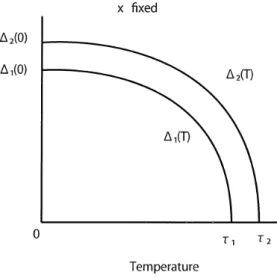
(4) 169 the simple gap equation (1.3) such that the solution \triangle_{1} is continuous, strictly decreasing with respect to the temperature T on the closed interval [ 0 , \mathcal{T}ı], and satisfies. \triangle_{1}(0)=\frac{\sqrt{(\hslash\omega_{D}-\varepsilone^{1/U_{1} ) (\hslash\omega_{D}-\varepsilone^{-1/U_{1)} {s\dot{ \imath} nh\frac{1}{U_{1} ,\triangle_{1}(\tau_{1})=0. Moreover, the solution \triangle_{1} is of class C^{2} with respect to the temperature. T. on the interval [0, \tau_{1} ). and. \triangle í(0). =\triangle_{1}"(0)=0,. T\uparow\tau_{\imath}1\dot{\imath}m. \triangle í. (T)=-\infty.. Remark 1.4. We set \triangle_{1}(T)=0 at T>\tau_{1} . See figure 1. x. fixed. \Delta_{2}(0) \Delta_{1}(0). 0. T_{\rceil} T_{2}. Temperature. Figure 1: The graphs of the functions \triangle_{1} and \triangle_{2} with. x. fixed.. We then introduce another positive constant U_{2}>0 . Let 0<U_{1}<U_{2} and set U(x, \xi)=U_{2} at all (x, \xi)\in[\varepsilon, \hslash\omega_{D}]^{2} . Then a simiıar discussion implies that for U_{2} , there is a unique. nonnegative solution \triangle_{2} : [0, \tau_{2}]arrow[0, \infty ) to the simple gap equation (1.5). 1=U_{2} \int_{\varepsilon}^{\hslash\omega_{D} \frac{1}{\sqrt{\xi^{2}+\triangle_ {2}(T)^{2} \tanh\frac{\sqrt{\xi^{2}+\triangle_{2}(T)^{2} {2T}d\xi, 0\leq T\leq \tau_{2}.. Here, \tau_{2}>0 is defined by. (1.6). 1=U_{2} \int_{\varepsilon}^{\hslash\omega_{D} \frac{1}{\xi}\tanh\frac{\xi} {2\tau_{2} d\xi.. Remark 1.5. We again set \triangle_{2}(T)=0 at T>\tau_{2}.. Lemma 1.6 ([14, Lemma 1.5]). (a) The inequality \tau_{1}<\tau_{2} holds. (b) If 0\leq T<\tau_{2} , then \triangle_{1}(T)<\triangle_{2}(T) . If T\geq\tau_{2} , then \triangle_{1}(T)=\triangle_{2}(T)=0..
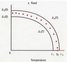
(5) 170 See figure 1. The function \triangle_{2} has properties similar to those of the function \triangle_{1}.. We define a nonlinear integral operator. (1.7). Au. A. by. (T, x)= \int_{\varepsilon}^{\hslash\omega_{D} \frac{U(x,\xi)u(T,\xi)} {\sqrt{\xi^{2}+u(T,\xi)^{2} \tanh\frac{\sqrt{\xi^{2}+u(T,\xi)^{2} {2T}d\xi.. Here the right side of this equality is exactly the right side of the BCS‐Bogoliubov gap equation. (1.2). Since the solution to the BCS‐Bogoliubov gap equation is a fixed point of our operator A,. we apply fixed point theorems to our operator A.. Let us turn to the BCS‐Bogoliubov gap equation (1.2). We assume the folıowing condition on the potential U(\cdot, \cdot) :. (1.8). U(\cdot, \cdot)\in C([\varepsilon, \hslash\omega_{D}]^{2}) ,. (0<)U_{1}\leq U(x, \xi)\leq U_{2}. at aıı. (x, \xi)\in[\varepsilon, \hslash\omega_{D}]^{2}.. Let 0\leq T\leq\tau_{2} and fix T . We now consider the Banach space C[0, \hslash\omega_{D}] consisting of continuous functions of the energy x only, and deal with the following temperature dependent subset V_{T} : V_{T}=. { u(T, \cdot)\in C[\varepsilon, hv_{D}] : \triangle_{1}(T)\leq u(T, x)\leq\triangle_{2}(T) at x\in[\varepsilon, \hslash\omega_{D}] }.. Remark 1.7. The set V_{T} depends on the temperature. T.. See figures 1 and 2.. We define our nonlinear integral operator A(1.7) on the set V_{T} . The foılowing gives another proof of the existence and uniqueness of the nonnegative solution to the BCS‐Bogoliubov gap equation, and shows how the solution varies with the temperature.. Theorem 1.8 ([14, Theorem 2.2]). Assume (1.8) and let T\in[0, \tau_{2}] be fixed. Then there is a uniqu e nonnegative solution u_{0}(T, \cdot)\in V_{T} to the BCS‐Bogoliubov gap equation (1.2):. u_{0}(T, x)= \int_{\varepsilon}^{\hslash x_{D} \frac{U(x,\xi)u_{0}(T,\xi)} {\sqrt{\xi^{2}+u_{0}(T,\xi)^{2} \tanh\frac{\sqrt{\xi^{2}+u_{0}(T,\xi)^{2} {2T} d\xi, x\in[\varepsilon, \hslash xv_{D}]. Consequently, the solution u_{0}(T, \cdot) with varies with the temperature as follows:. T. fixed is continuous with respect to the energy. \triangle_{1}(T)\leq u_{0}(T, x)\leq\triangle_{2}(T). at. x. and. (T, x)\in[0, \tau_{2}]\cross[\varepsilon, \hslash\omega_{D}].. See figure 2. Remark 1.9. Let u_{0}(T, \cdot) be the solution as in Theorem 1.8. If there is a point x_{1}\in[\varepsilon, \hslash u_{D}] satisfying u_{0}(T, x_{1})=0 , then u_{0}(T, x)=0 at all x\in[\varepsilon, \hslash u_{D}] . See [14, Proposition 2.4].. The existence and uniqueness of the transition temperature T_{c} were pointed out in previous. papers [5, 6, 7, 13]. In our case, we can define it as folıows: Definition 1.10. Let u_{0}(T, \cdot) be the solution given by Theorem 1.8. temperature T_{c} is defined by T_{c}= \inf { T>0:u_{0}(T, x)=0. at all. Then the transition. x\in[\varepsilon, \hslash\omega_{D}] }.. Remark 1.11. Let u_{0}(T, \cdot) be the solution given by Theorem 1.8. At T\geq T_{c} , we set u_{0}(T, x)=0 at all x\in[\varepsilon, \hslash a_{D}] . The transition temperature T_{c} is the critical temperature that divides normal conductivity and superconductivity, and satisfies \tau_{1}\leq T_{c}\leq\tau_{2} . See figure 2..
(6) 171 171 x. fixed. A_{2}(0) \Delta,(0). Temperature. Figure 2: For each fixed. T,. the solution u_{0}(T, x) is between \triangle_{1}(T) and \triangle_{2}(T) .. But Theorem 1.8 tells us nothing about continuity and smoothness of the solution. u_{0}. with. respect to the temperature T . Applying the Banach fixed‐point theorem, we then showed in [15, Theorem 1.2] that the solution u_{0} is indeed continuous both with respect to the temperature T. and with respect to the energy. x. under the restriction that the temperature. small. See also [16]. Let us denote by z_{0}>0 a unique solution to the equation z_{0}. is nearly equal to 2.07. Let \tau 0(>0) satisfy. (1.9). \frac{2}{z}=\tanh z. T. is sufficiently. (z>0) . Note that. \triangle_{1}(\tau_{0})=2z_{0}\tau_{0}.. From (1.9) it follows immediately that (0<)\tau_{0}<\tau_{1}. Remark 1.12. Observed values in many experiments by using superconductors imply the tem‐ perature \tau_{0} is nearly equal to T_{c}/2. Let 0<\tau_{3}<\tau_{0} and fix. C([0, \tau_{3}]\cross[\varepsilon, \hslash\omega_{D}]) V. =. \tau_{3} .. We then deal with the foılowing subset. V. of the Banach space. :. \{u\in C([0, \tau_{3}]\cross[\varepsilon, \hslash\omega_{D}]) : 0\leq u(T, x)-u(T', x)\leq\gamma(T'-T) \triangle_{1}(T)\leq u(T, x)\leq\triangle_{2}(T),. u. (T<T') ,. is partially differentiable with respect to. T. twice,. \frac{\partial u}{\partial T}, \frac{\partial^{2}u}{\partial T^{2} \in C([0, \tau_{3}]\cros [\varepsilon, \hslash xv_{D}])\}. Here, see [17, (2.2)] for the positive constant \gamma>0 . We define our operator (1.7) on the subset V. We denote by \overline{V} the closure of the subset. C([0, \tau_{3}]\cross[\varepsilon, \hslash\omega_{D}]). V. with respect to the norm of the Banach space. .. Theorem 1.13 ([17, Theorem 1.10]). Assume (1.8). Then the operator A:\overline{V}arrow\overline{V} has a unique. fixed point u_{0}\in\overline{V}, and so there is a unique nonnegative solution u_{0}\in\overline{V} to the BCS‐Bogoliubov. gap equation (1.2):. u_{0}(T, x)= \int_{\varepsilon}^{\hslash\omega_{D}. anh. \frac{\sqrt{\xi^{2}+u_{0}(T,\xi)^{2} }{2T}d\xi,. 0\leq T\leq\tau_{3},. \varepsilon\leq x\leq\hslash\omega_{D}..
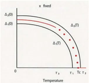
(7) 172 Consequently, the solution u_{0} is continuous on [0, \tau_{3}]\cross[\varepsilon, \hslash u_{D}] , i. e., the solution u_{0} is continuous with respect to both the temperature T and the energy x . Moreover, the solution u_{0} is Lipschitz continuous and monotone decreasing with respect to the temperature T , and satisfies \triangle_{1}(T)\leq u_{0}(T, x)\leq\triangle_{2}(T) at all (T, x)\in[0, \tau_{3}]\cross[\varepsilon, \hslash u_{D}] . Furthermore, if u_{0}\in V , then the solution u_{0} is partially differentiable with respect to the temperature T twice and the second‐order partial derivative is continuous with respect to both the temperature T and the energy x . On the other hand, if u_{0}\in\overline{V}\backslash V , then the solution u_{0} is approximated by such a smooth element of the subset V with respect to the norm of the Banach space C([0, \tau_{3}]\cross[\varepsilon, \hslash\omega_{D}]) .. See figure 3 for the graph of the solution. x. u_{0}. with the energy. x. fixed.. fixed. \Delta_{2}(0) \Delta_{t}(0). \vee O - \cdot. Temperature Figure 3: The solution. 2. u_{0}. belongs to the subset \overline{V}.. Main results. We choose an arbitrary. \tau>0. satisfying \tau_{1}<\tau<\tau_{2}.. Here, \tau_{1}>0 (resp. \tau_{2}>0 ) is reıated to U{\imath}>0 by (1.4) (resp. to U_{2}>0 by (1.6)). Let the potential U(\cdot, \cdot) satisfy (1.8) and the following: (2.1). (0<)a= \max_{x\in[\varepsilon,\hslash\omega_{D}] (\int_{\varepsilon}^{n_{A_{D} }\frac{U(x,\xi)}{\xi}\tanh\frac{\xi}{2\tau}d\xi)<1.. Even when the potential U(\cdot, \cdot) satisfies both (1.8) and (2.1), Theorem 1.8 again implies that there is a unique nonnegative solution u_{0}(T, \cdot)\in V_{T} to the BCS‐Bogoliubov gap equation (1.2)..
(8) 173 By Definition 1.10, the transition temperature T_{c}>0 is thus defined. Note that the transition temperature T_{c}>0 is related to the solution u_{0}(T, \cdot)\in V_{T} . As for the relation between \tau and T_{c} , we have \tau<T_{c} or \tau\geq T_{c} . So we choose the potential such that the relation \tau<T_{c} holds true, and we then consider the soıution u_{0}(\cdot, \cdot) to the BCS‐Bogoliubov gap equation defined on. [\tau, T_{c}]\cross[\varepsilon, \hslash f_{\lrcorner}J_{D}]. Let us consider the following condition, which gives the behavior of the solution u_{0}(\cdot, \cdot) to the BCS‐Bogoliubov gap equation as T\uparrow T_{c} :. Condition (C). An element u\in C([\tau, T_{c}]\cross[\varepsilon, \hslash\omega_{D}]) is partially differentiable with respect to the temperature T\in[\tau, T_{c} ) twice, and both (\partial u/\partial T) and (\partial^{2}u/\partial T^{2}) belong to C([\tau, T_{c} ) \cross [\varepsilon, \hslash u_{D}]) . Moreover, for the u above, there are a unique v\in C[e, \hslash\omega_{D}] and a unique w\in C[\varepsilon, \hslash\omega_{D}] satisfying the following: (C1) v(x)>0 at all x\in[\varepsilon, \hslash x_{A}) D ]. (C2) For an arbitrary \varepsilon_{1}>0 , there is a \delta>0 such that |T_{c}-T|<\delta implies. |v(x)- \frac{u(T,x)^{2} {T_{c}-T}|<T_{c}\varepsilon_{1}. |v(x)+2u(T, x) \frac{\partial u}{\partial T}(T, x)|<T_{c}\varepsilon_{1}.. and. \delta does not depend on x\in[\varepsilon, \hslash\omega_{D}]. (C3) For an arbitrary \varepsilon_{1}>0 , there is a \delta>0 such that |T. -T|<\delta implies. Here, the. | \frac{w(x)}{2}+\frac{u(T,x)^{2}+(T_{c}-T)\frac{\partial}{\partial T}\{u(T,x)^ {2}\} {(T_{c}-T)^{2} |<\varepsilon_{1}. and. |w(x)- \frac{\partial^{2} {\partial T^{2} \{u(T, x)^{2}\}|<\varepsilon_{1}.. Here, the \delta does not depend on x\in[\varepsilon, \hslash\omega_{D}].. Remark 2.1. Conditions (C2) and (C3) imply. T \upar ow T_{c}{\imath} im\frac{\partial u(T,x)^{2} {\partial T}=-v(x). and. Each of them converges uniformly with respect to Consider a subset W. =. W. T \upar ow T_{c}1\dot{ \imath} m\frac{\partial^{2}u(T,x)^{2} {\partial T^{2} =w (x). .. x.. of the Banach space C([\tau, T_{c}]\cross[\varepsilon, \hslash\omega_{D}]) :. u(T, x)\geq u(T', x)(T<T') , 0=\triangle_{1}(T)\leq u(T, x)\leq\triangle_{2}(T) at (T, x), (T', x)\in[\tau, T_{c}]\cross[\varepsilon, \hslash u_{D}],. \{u\in C([\tau, T_{c}]\cross[\varepsilon, \hslash\omega_{D}]) u. :. satisfies Condition (C) above}.. We then define a nonlinear integral operator A(1.7) on the closure \overline{W} of the subset W , and ıook for a fixed point in \overline{W} of our operator A . Here, \overline{W} denotes the closure of the subset W with respect to the norm of the Banach space C([\tau, T_{c}]\cross[\varepsilon, \hslash\omega_{D}]) .. Remark 2.2. It follows directly from Condition (C2) that u(T_{c}, x)=0 at all x\in[\varepsilon, \hslash\omega_{D}] for u\in W.. One of our main results is the following:. Theorem 2.3. Choose the potential U(\cdot, \cdot) such that U(\cdot, \cdot) satisfies (1.8), (2.1) and the relation \tau<T_{c} .. Then the operator. A. : \overline{W}arrow\overline{W} is contractive, and so there is a unique fixed point. u_{0}\in\overline{W} of the operator A : \overline{W}arrow\overline{W} . Consequently, there is a unique nonnegative solution u_{0}\in\overline{W} to the BCS‐Bogoliubov gap equation (1.2):. u_{0}(T, x)= \int_{\varepsilon}^{\hslash\omega_{D} \frac{U(x,\xi)u_{0}(T,\xi)}{ \sqrt{\xi^{2}+u_{0}(T,\xi)^{2} \tanh\frac{\sqrt{\xi^{2}+u_{0}(T,\xi)^{2} {2T}d \xi,. \tau\leq T\leq T_{c}. ,. \varepsilon\leq x\leq\hslash\omega_{D}..
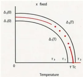
(9) 174 The solution u_{0} is continuous on [\tau, T_{c}]\cross[\varepsilon, \hslash\omega_{D}] and is monotone decreasing with respect to the temperature T. Moreover, the solution u_{0} satisfies that 0=\triangle_{1}(T)\leq u(T, x)\leq\triangle_{2}(T) at all (T, x)\in[\tau, T_{c}]\cross[\varepsilon, \hslash\omega_{D}] and that u_{0}(T_{c}, x)=0 at all x\in[\varepsilon, \hslash\omega_{D}] . If u_{0}\in W , then the. solution. u_{0}. is smooth with respect to the temperature. ifu_{0}\in\overline{W}\backslash W , then the solution. u_{0}. T. and satisfies Condition (C) . Furthermore,. is approximated by a smooth element of the subset. W. fulfilling. Condition (C) . See figure 4 for the graph of the solution energy x fixed.. x. u_{0}. near the transition temperature T_{c} with the. fixed. \Delta_{2}(0) \Delta,(0). Temperature. Figure 4: The graph of the solution. Approximation (A). The function. u. u_{0}. near the transition temperature T_{c}.. in \Psi(1.1) is the solution u_{0}\in\overline{W} of Theorem 2.3.. However, if the solution is in the set \overline{W}\backslash W , then the solution u_{0} might not be differentiable with respect to the temperature T . This means that \Psi(1.1) might not be differentiable with respect to the temperature T . We then approximate the solution u_{0}\in\overline{W}\backslash W by a suitably u_{0}. chosen element u_{1}\in W , and we replace the function u in (1.1) by this element u_{1}\in W . In \Psi (1.1) we thus use this element u_{1}\in W instead of the solution u_{0}\in\overline{W}\backslash W . Accordingly, we consider the functions v and w in Condition (C) as those corresponding to this element u_{1}\in W. In this way, we can differentiate this element u_{1}\in W with respect to the temperature T twice, and hence \Psi(1.1) with respect to the temperature T twice. On the other hand, if the solution u_{0} of Theorem 2.3 is in the subset W , then the solution u_{0} is differentiable with respect to the temperature T twice. Needless to say, in this case, we use the solution u_{0}\in W instead of this element u_{1}\in W , and we need no approximation in this case.. We can show that all the conditions of Definition 1.1 hold true. We thus obtain the following:. Theorem 2.4. Assume Approximation (A) if necessary. Then the transition to a superconduct‐ ing state at the transition temperature T_{c} is a second‐order phase transition..
(10) 175 Let. g. Note that. : [0, \infty)arrow \mathbb{R} be given by. g(\eta)=\{begin{ar y}{l \frac{1}\eta^{2}\cosh^{2}\eta}-\frac{\tanh\eta}{\eta^{3} (\eta>0), -\frac{2}3 (\eta=0). \end{ar y}. g(\eta)<0.. We have one more main result:. Theorem 2.5. Assume Approximation (A) if necessary. Let. v. and. g. be as above. Then the gap. \triangle C_{V} in the specific heat at constant volume at the transition temperature T_{c} is given by. \triangle C_{V}=-\frac{N_{0} {8T_{c} \int_{\varepsilon/(2T_{c}) ^{\hslash_{Ad_ {D} /(2T_{c}) v(2T_{c}\eta)^{2}g(\eta)d\eta (>0) Remark 2.6. Putting. \varepsilon=0. (2.2). .. gives. \triangle C_{V}=-\frac{N_{0} {8T_{c} \int_{0}^{\hslash\omega_{D}/(2T_{c})} v(2T_{c}\eta)^{2}g(\eta)d\eta (>0). .. Remark 2.7. If the potential U(\cdot, \cdot) of the BCS‐Bogoliubov gap equation (1.2) is a positive constant, then putting. \varepsilon=0. (2.3). gives. \triangle C_{V}=N_{0}v\tanh\frac{\hslash\omega_{D} {2k_{B}T_{c} (>0) .. Remark 2.8. If the potential U(\cdot, \cdot) of the BCS‐Bogoliubov gap equation is not a constant but a function, then we have (2.2). On the other hand, if the potential U(\cdot, \cdot) is reduced to a. constant, then we have (2.3). As far as the present author knows, no one obtained (2.2) and no one obtained (2.3). In previous physics literature, one obtained only an approximate expression that approximates (2.3). But, this time, we obtain the exact and explicit expression (2.2) from the viewpoint of operator theory.. Acknowledgments S. Watanabe is supported in part by the JSPS Grant‐in‐Aid for Scientific Research (C) 24540112. References. [1] V. Bach, E. H. Lieb and J. P. Solovej, Generalized Hartree‐Fock theory and the Hubbard model, J. Stat. Phys. 76 (1994), 3‐89. [2] J. Bardeen, L. N. Cooper and J. R. Schrieffer, Theory of superconductivity, Phys. Rev. 108 (1957), 1175‐1204. [3] P. Billard and G. Fano, An existence proof for the gap equation in the superconductivity theory, Commun. Math. Phys. 10 (1968), 274‐279..
(11) 176 [4] N. N. Bogoliubov, A new method in the theory of superconductivity I, Soviet Phys. JETP 34 (1958), 41‐46.. [5] R. L. Frank, C. Hainzl, S. Naboko and R. Seiringer, The critical temperature for the BCS equation at weak coupling, J. Geom. Anal. 17 (2007), 559‐568. [6] C. Hainzl, E. Hamza, R. Seiringer and J. P. Solovej, The BCS functional for general pair interactions, Commun. Math. Phys. 281 (2008), 349‐367. [7] C. Hainzl and R. Seiringer, Critical temperature and energy gap for the BCS equation, Phys. Rev. B77 (2008), 184517.. [8] A. L. Kuzemsky, Bogoliubov’s vision: quasiaverages and broken symmetry to quantum pro‐ tectorate and emergence, Internat. J. Mod. Phys. B, 24 (2010), 835‐935. [9] A. L. Kuzemsky, Variational principle of Bogoliubov and generalized mean fields in many‐ particle interacting systems, Internat. J. Mod. Phys. B, 29 (2015), 1530010 (63 pages). [10] A. L. Kuzemsky, Statistical Mechanics and the Physics of Many‐Particle Model Systems, World Scientific Publishing Co., Singapore, 2017.. [11] M. Niwa, Fundamentals of Superconductivity, Tokyo Denki University Press, Tokyo, 2002 (in Japanese). [12] F. Odeh, An existence theorem for the BCS integral equation, IBM J. Res. Develop. 8 (1964), 187‐188. [13] A. Vansevenant, The gap equation in the superconductivity theory, Physica 17D (1985), 339‐344.. [14] S. Watanabe, The solution to the BCS gap equation and the second‐order phase transition in superconductivity, J. Math. Anal. Appl. 383 (2011), 353‐364. [15] S. Watanabe, Addendum to ‘The solution to the BCS gap equation and the second‐order phase transition in superconductivity’, J. Math. Anal. Appl. 405 (2013), 742‐745. [16] S. Watanabe, An operator‐theoretical treatment of the Maskawa‐Nakajima equation in the massless abelian gluon model, J. Math. Anal. Appl. 418 (2014), 874‐883. [17] S. Watanabe and K. Kuriyama, Smoothness and monotone decreasingness of the solution to the BCS‐Bogoliubov gap equation for superconductivity, J. Basic Appl. Sci. 13 (2017), 17‐25.. [18] J. M. Ziman, Principles of the Theory of Solids, Cambridge University Press, Cambridge, 1972..
(12)
図
関連したドキュメント
The torsion free generalized connection is determined and its coefficients are obtained under condition that the metric structure is parallel or recurrent.. The Einstein-Yang
In this section, we establish some uniform-in-time energy estimates of the solu- tion under the condition α − F 3 c 0 > 0, based on which the exponential decay rate of the
In this note, we consider a second order multivalued iterative equation, and the result on decreasing solutions is given.. Equation (1) has been studied extensively on the
Evtukhov, Asymptotic representations of solutions of a certain class of second-order nonlinear differential equations..
We consider the global existence and asymptotic behavior of solution of second-order nonlinear impulsive differential equations.. 2000 Mathematics
Gupta, “Solvability of a three-point nonlinear boundary value problem for a second order ordinary differential equation,” Journal of Mathematical Analysis and Applications,
Inside this class, we identify a new subclass of Liouvillian integrable systems, under suitable conditions such Liouvillian integrable systems can have at most one limit cycle, and
Theorem 2.11. Let A and B be two random matrix ensembles which are asymptotically free. In contrast to the first order case, we have now to run over two disjoint cycles in the
