Bifurcation analysis to Rayleigh-Benard convection at degenerate critical points (Mathematical Analysis in Fluid and Gas Dynamics)

Bifurcation analysis

to

Rayleigh-B\’enard

convection at degenerate

critical

points

大阪大学・大学院基礎工学研究科 小川知之 (Toshiyuki Ogawa)

GraduateSchool of Engineering Science

Osaka University

1

Introduction

In this paper

we

consider pattern formation problem to the classical Rayleigh-Benard

con-vection by the standard bifurcation analysis method. Let

us

consider the problem by the

Bussinesq approximation (Oberbeck-Boussinesq model) with

_uP-down

symmetric boundary

condition. It is already a classical fact that the hexagonal pattern appear right after the

critical Rayleigh number and it is unstable. See forexample [6]. In [2] theyobtained general

bifurcational structure under the

uP-down

symmetryincludingtheBoussinesq approximation.

However, both of them have not obtained the eigenvalues about the mixed mode solutions

such

as

the hexagonal pattern. On the other hand, recent $3\mathrm{D}$ numerical simulation shows

that it is rather easy to obtain the hexagonal pattern under the

same

_uP-down

symmetric

situation $(\mathrm{e}\mathrm{g}$

.

[3]$)$

.

Therefore

we

have calculated the cubic normal form about the critical

point where both the roll and hexagonal patterns appearand study the dynamics ofthem in

our

previous study([5]). By the cubic normal form we

can

study the invariant torus which

includes the fixed point corresponding to the hexagonal pattern inside. To determine the

motion on the torus

we

need to calculate the normalform up to higher order. But we only

discuss the stabilityof the invariant torus and calculatetheeigenvalues for the transversal

di-rection tothetorus. Oneof

our

previous results shows that it istrue thatthe invariant torus

ofthehexagonal patternhas positiveeigenvalues but they

are

smallcompared totheabsolute

value of thenegative

ones.

The invarianttorus is

a

saddle for its transversal directions and

it will take quite

a

long time to observe unstable dynamics. It is consistent to the classical

theoretical results and also the numerical simulations. Notice that a hexagonal pattern

can

be stable in the

case

when the two boundary condition

are

different so that it breaks the

uP-down

symmetry. In fact the normal form has quadratic terms which correspond to the

hexagonal

resonance.

In these previous works the fluid tank with particular size is mainly considered. There

exist 3 roll solutions which have the

same

critical

wave

length and

cross

each other by the

angleof120 degrees. Here; inthis study,

we

shall consider

more

generalsituationsby changing

the size of the tank. It is still difficult to study the reduce dynamics for all the variations of

the system size. However,

we

found astable mixed mode solution (patchwork quilt tyPe) by

taking the size and the Prandtl number appropriately.

2

Formulation

We consider the Boussinesq approximation for the Rayleigh-Benard convection. Variation

equations about the conductive state

can

be written in the following non-dimensional form.

$\{$

$u_{t}+$ (tt

.

$\nabla$)_{$u$ $=$}

$\theta_{t}+(u\cdot\nabla)\theta$ $=$

$\nabla\cdot u$ $=$

$-\nabla p+R\theta \mathrm{e}_{z}+$ Au

$(w+\Delta\theta)/P$ (2.1)

Here, $u=(u,v,w)$ is

a

velocity vector and $\mathrm{e}_{z}=(0, 0,1)$. Two constants $R$ and $P$

are

the

Rayleigh and the Prandtl numbers, $1^{\backslash }\mathrm{e}\mathrm{s}\mathrm{p}\mathrm{e}\mathrm{c}\mathrm{t}\mathrm{i}\mathrm{v}\mathrm{e}1\mathrm{y}$.

Let the boundary conditions be free-slipfor both the top and the bottom:

$u_{z}=v_{z}=w=\theta=0$ $(z =0, 1)$. (2.2)

Therefore solutions to this problem have

uP-down

symmetry which

means

that they

are

invariant under the mapping:

$(u_{;}v, w, \theta,p)(t_{;}x,y, z)\mapsto(u, v, -w, -\theta,p)(t,x, y, 1-z)$.

Moreover let

us

assumethe periodlcity for both$x$and$y$directions with the

$\mathrm{p}\mathrm{e}\mathrm{l}\cdot \mathrm{i}\mathrm{o}\mathrm{d}\mathrm{s}$ $(2\pi/\alpha,2\pi/\beta)$.

We represent each unknownvariables by the Fourier expansion.

$u= \sum_{\langle m,n,l)\in \mathrm{Z}^{3}}u_{m,’ x},\iota e^{i(m\alpha x+n\beta y+l\pi z)}$

We

use

an abrebiated

notation $\mathrm{m}=(n\iota,n, l)$ for the mode vector and $u_{\mathrm{m}}=u_{m,n,l}$. Since all theunknown variables

are

real valued and their Fouriercoefficientshave the

Her-mitian symmetry: $u_{\mathrm{r}\mathrm{n}}=u_{-f\mathrm{n}}$

.

They also satisfy the following properties which correspond

to the up-down symmetry.

$u_{m,n,l}$ $=$ $u_{m,n,-l}$, $v_{m,n,l}$ $=$ $v_{m,n,-l;}$ (2.3) $w_{m,n},\iota$ $=$ $-w_{7n,n,-l;}$ $\theta_{m,n,l}$ $=$ $-\theta_{m,n,-l}$

,

$Pm,n,l$ $=$ $p_{m,n,-}\iota$

Now

we

rewrite the equations $(2,1)$ by using the Fouriercoefficients $\mathrm{a}_{1}\mathrm{s}$ follows.

$(\begin{array}{l}u_{\dot{\mathrm{I}}\mathrm{n}}v_{\dot{\mathrm{m}}}u^{j_{\mathrm{m}}}\theta_{\dot{\mathrm{m}}}0\end{array})=($

$-\omega^{2}000$ $-\omega^{2}000$ $-\omega^{2}1/P00$

$-\omega_{0}^{2}/PR00$ $-\mathrm{i}n\iota\alpha-\mathrm{i}n\beta-\dot{\uparrow,}l\pi 00)$

$(\begin{array}{l}u_{\mathrm{m}}v_{\mathrm{m}}w_{\mathrm{m}}\theta_{\mathrm{m}}p_{\mathrm{m}}\end{array})-(\begin{array}{l}\{(u\cdot\nabla)u\}_{\mathrm{m}}\{(u\cdot\nabla)v\}_{\mathrm{m}}\{(u\cdot\nabla)w\}_{\mathrm{m}}\{(u\cdot\nabla)\theta\}_{\mathrm{m}}0\end{array})$ (2.4)

$im\alpha$ $in\beta$ $il\pi$

Here, $\omega^{2}=m^{2}\alpha^{2}+n^{2}\beta^{2}+l^{2}\pi^{2}$.

(2.4) with the symmetry (2.3) is equivalent to (2.1) with (2.2). Moreover the Fourier

coefficients for the

pressure

$p$ and $w$

can

be eliminated by the fifth equation of (2.4) and

finally

we

obtain the following system ofordinary

differential

equations for $\mathrm{m}\neq 0$

.

$(\begin{array}{l}u_{\dot{\mathrm{m}}}v_{\dot{\mathrm{m}}}\theta_{\dot{\mathrm{m}}}\end{array})=M_{\mathrm{m}}$

$(\begin{array}{l}\prime U\prime \mathrm{m}v_{\mathrm{m}}\theta_{\mathrm{m}}\end{array})-(\begin{array}{l}\{(u \cdot \nabla)u\}_{\mathrm{m}}\{(u\cdot\nabla)v\}_{\mathrm{m}}\{(u\cdot\nabla)\theta\}_{\mathrm{m}}\end{array})$ $+k_{\mathrm{m}}$

$(\begin{array}{l}?\uparrow]\alpha n\beta 0\end{array})$

$(l \neq 0)$ (2.5)

$(\begin{array}{l}u_{\dot{\mathrm{m}}}v_{\dot{\mathrm{m}}}\end{array})=M_{(m,n\}0)}$

$(\begin{array}{l}u_{\mathrm{m}}v_{\mathrm{m}}\end{array})-(\begin{array}{l}\{(u\cdot\nabla)u\}_{\mathrm{m}}\{(u\cdot\nabla)v\}_{\mathrm{m}}\end{array})$ $+k_{(m,n,0)}$

$(\begin{array}{l}m\alpha n\beta\end{array})$ ($l=0$ and $\mathrm{m}\neq 0$)

(2.6) Here,

$M_{r\mathrm{n}}=(\begin{array}{lll}-\omega^{2} 0 -77\mathrm{k}l\pi\alpha R/\omega^{2}0 -\omega^{2} -nl\pi\beta R/\omega^{2}-m\alpha/l\pi P -n\beta/l\pi P -\omega^{2}/P\end{array})$ , $(l\neq 0)$,

$M_{\mathrm{m}}=(\begin{array}{ll}-\omega^{2} 0\mathrm{O} -\omega^{2}\end{array})$ , ($f=0$ and $\mathrm{m}\neq 0$)

Notice that the

mean

flow should be zero, that is $u_{0}=v0$ $=Po=0$ and it holds that

$w_{0}=\theta_{0}=0$ by the symm etry (2.3). It is easy to

see

that the linearized matrix $M_{\mathrm{m}}$ has

0-eigenvalue ifand only if$l\neq 0$ and $R=R(k)=(k^{2}+l^{2}\pi^{2})^{3}/k^{2}$where$k$ isthe wave number

with $k^{2}=\uparrow 7\iota^{2}\alpha^{2}+n^{2}\beta^{2}$. $R(k)$ takesits minimumvalue$R_{c}=27\pi^{4}/4$at thecritical wavelength

$k_{c}=\sqrt{2}\pi/2$. $R_{\mathrm{c}}$ is called the critical Rayleigh number. We

axe

interested in the

case

when

the first instability takes place

as

weincrease the Rayleigh number. Therefore, we have only

to consider the

case

$l=1$ and $R=R(k)$ $=(k^{2}+\pi^{2})^{3}/k^{2}$.

Let

us

similarly consider the2dimensional

case

wherethe solution depends onlyon$(x, z)-$

direction. Now the unknown variables

are

$u$,$w$,$\theta,p$and theirtimeevolution

can

bedescribed

as

follows. Notice that the modevector is $\mathrm{m}=(m, l)\in \mathrm{z}^{2}$ and $\omega^{2}=m^{2}\alpha^{2}+l^{2}\pi^{2}$.

$(\begin{array}{l}u_{\mathrm{m}}\backslash \theta_{\dot{\mathrm{m}}}\end{array})=M_{\mathrm{m}}$ $(\begin{array}{ll}u_{\mathrm{m}} \theta_{\mathrm{m}} \prime\end{array})-(\begin{array}{l}\{(u\cdot\nabla)u\}_{\mathrm{m}}\{(u\cdot\nabla)\theta\}_{\mathrm{m}}\end{array})\backslash$

,

$+k_{\mathrm{m}}($ $m_{0}\alpha,)$ $(l\neq 0)$ (2.7)

$u_{\dot{\mathrm{m}}}=-\omega^{2}u_{\mathrm{m}}$ (l $=0$ and m$\neq 0$) (2.8)

Here, $M_{\mathrm{m}}$ and $k_{\mathrm{m}}$

are

defined

as

follows although we

use

the

same

notation

as

the3-D

case.

$k_{\mathrm{m}}= \frac{1}{\omega^{2}}(m\alpha\{(u. \nabla)u\}_{\mathrm{n}1}+l\pi\{(u\cdot\nabla)u)\}_{\mathrm{m}})$,

$l\mathrm{t}’I_{\mathrm{m}}=(\begin{array}{ll}-\omega^{2} -ml\pi\alpha R/\omega^{2}-m\alpha/l\pi P -\omega^{2}/P\end{array})$, $(l\neq 0)$

Now let

us

calculate the convolution terms.

$\{(u. \nabla)u\}_{\mathrm{m}}$

$=$

$\mathrm{m}_{1}+\mathrm{m}_{2}=\mathrm{m}\sum_{l_{1}\neq 0}\frac{\mathrm{i}\alpha(m_{2}l_{1}-m_{1}l_{2})}{l_{1}}u_{\mathrm{m}_{1}}u_{[] \mathrm{n}_{2}}$ (2.9)

$\{(u.\nabla)\theta\}_{\mathrm{m}}$

$=$

$\mathrm{m}_{1}+\mathrm{m}_{2}=\mathrm{m}\sum_{l_{1}\neq 0}\frac{i\alpha(m_{2}f_{1}-m_{1}l_{2})}{l_{1}}u_{\mathrm{m}_{1}}\theta_{\mathrm{m}_{2}}$ (2.10)

$\{(u\cdot\nabla)w\}_{\mathrm{m}}$ $=$

$\mathrm{m}_{1}+\mathrm{m}_{2}=\mathrm{m}\sum_{l_{1}l_{2}\neq 0}-\frac{\mathrm{i}m_{2}\alpha^{2}(n\tau_{2}l_{1}-l7?_{1}l_{2})}{l_{1}l_{2}\pi},u_{\mathrm{m}1}u_{\mathrm{m}_{2}}$ (2.11)

Here, we denote $\mathrm{m}_{i}=(m_{i}, l_{i})$.

These coupled systems $( (2,5)$ (2.6) and (2.7) (2.8) $)$ of countably many ordinary

differ-ential equations have

a

trivial

zero

solution. We study the local bifurcation about the trivial

solution. It is necessary to calculate the normal form

on

the center manifold which is locally

spanned by thecritical eigenvectors of$M_{\mathrm{m}}$ foreach set ofparameter values of$(R, \alpha, \beta)$.

There

are

two possibilities of critical points in the 2-D

case.

In fact if

a

critical point

is degenerate then two adjacent modes , $n$ and $n+1$ modes, are critical. In the 3-D case,

if

we

choose the domain with $(\alpha,\beta)$ $=k_{c}(1/2, \sqrt{3}/2)$ where $k_{c}$ is the critical

wave

length, 3

critical modes appear and they correspond to the roll patterns which differ by 120 degrees

3

2-D

problem

and

stability

of

mixed

mode solutions

We review

our

previousresultsforthe stability of mixed mode solutionsfor a2-D fluid tank.

It might be easier to explain

our

analysis in the 2-D problem and

we

basically take similar

strategy for the 3-D problem.

When $R=R(\alpha;m):=(n\iota^{2}\alpha^{2}+\pi^{2})^{3}/m^{2}\alpha^{2}$ holds, $(m1)\}$ mode becom

es

critical in the

linearized problem about

zero

to (2.7)(2.8). Therefore at most two critical modes become

critical at the

same

time. Moreprecisely, for

a

given athere exists

a

number $R^{*}$ such that all

the eigenvalues about

zero

is negative for $R<R^{*}$) and

moreover one

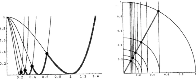
of the following holds.

(See also Figure 1.)

:

.

simple critical

case:

There exists

a

natural number $n$ such that $R^{*}=R(\alpha;\pm n, 1)$

and if $|?71|\neq n$ then $R^{*}<R(\alpha;m, 1)$. We call the pair of parameter values $(\alpha, R^{*})\mathrm{a}$

simple critical point.

.

multiple critical case: Thereexistsa natural number$n$such that $R^{*}=R(\alpha;\pm n, 1)=$

$R(\alpha;\pm(n+1), 1)$ and if $|m|\neq n$,$n+1$ then $R^{*}<R(\alpha,\cdot m, 1)$. We call the pair of

parameter values $(\alpha, R^{*})$

a

multiple critical point.

Figure 1: [Left $\mathrm{f}\mathrm{i}\mathrm{g}\mathrm{u}\mathrm{r}\mathrm{e}|:\mathrm{N}\mathrm{e}\mathrm{u}\mathrm{t}\mathrm{r}\mathrm{a}\mathrm{l}$stability

curves

drawn in

$(\alpha, \#)$-plane. They correspond

the critical

curves

for $R$ $=$ $R(\alpha;1)$, $\cdots$ ,$R(\alpha, 4)$ respectively from the right. Thick

curve means

the first instability and the black dots

are

mutiple critical points. [Right

$\mathrm{f}\mathrm{i}\mathrm{g}\mathrm{u}\mathrm{r}\mathrm{e}]:C_{m,\mathrm{n}}$ drawn in $(\alpha,\beta)$-plane for the 3-D problem (See section 4 in detail)

for

$(m, n)$ $=(1_{7}1)$,$(2, 2)$,$(3, 3)$, $(4, 4)$,$(5, 5)$,$(2, 0)$, $(3, 0)$,$(4, 0)$,$(5, 0)$,$(6, 0)$,$(7, 0)$,$(8, 0)$,$(9, 0)$ and $(10, 0)$_. Black dots correspond to the hexagonal critical points.

It is easy to

see

that a roll solution bifurcates at

a

simple

critical

point

as

a

super-critical pitchfork bifurcation. In fact, $M_{\mathrm{m}}$ has simple $0$-eigenvalue ifand only if

$\mathrm{m}\in S.=$

$\{(\pm n, \pm 1), (\pm n, \mp 1)\}$. Thecritical eigenvectors

are

not $v_{\mathrm{m}}$ but time.

$\mathrm{m}\in S$

as

follows. The

linear transformation:

$(\begin{array}{l}\tilde{u}\mathrm{m}\tilde{\theta}_{\mathrm{m}}\end{array})=T$ $(\begin{array}{l}u_{\mathrm{m}}\theta_{\mathrm{m}}\end{array})$ , $T= \frac{1}{(1+P)_{l71}\alpha l\pi\omega^{2}}$

make the linear part of the equation for $\mathrm{m}\in S$ diagonal

as

$(\begin{array}{l}\tilde{u}_{\dot{\mathrm{m}}}\overline{\theta}_{\dot{\mathrm{m}}}\end{array})=(\begin{array}{ll}0 00 -\frac{1+P}{P}\omega^{2}\end{array})(\begin{array}{l}\tilde{u}_{\mathrm{m}}\tilde{\theta}_{\mathrm{m}}\end{array})$ $-T$ $(\begin{array}{l}\{(u\cdot\nabla)u\}_{\mathrm{m}}\{(u\cdot\nabla)\theta\}_{\mathrm{I}\mathrm{n}}\end{array})$$+Tk_{\mathrm{m}}$ $(\begin{array}{l}n\uparrow\alpha 0\end{array})$ (3.1)

Now the center manifold about the simple critical point

can

be described by $\tilde{u}_{\mathrm{m}}(\mathrm{m}\in S)$

.

The other modes: $\overline{\theta}_{\mathrm{m}}(\mathrm{m}\in S)$ and $u_{\mathrm{m}\}}\theta_{\mathrm{m}}(\mathrm{m}. \not\in S)$

are

the slave modes. Moreover, it

holds that $\tilde{u}(n_{l}1)=\tilde{u}(n,-1)$ by the up-down symmetry. Therefore $\overline{u}\langle n,1$),$\overline{\tilde{u}(n,1)}$ gives the local

coordinate

on

the center manifold. We

are

interested in the small solutions $|\tilde{u}(n,1)|<\delta$

near

the critical point. Then all the slave modes are $O(\delta^{2})$ by the center manifold theorem. To

obtain the effective normal formon thecenter manifold

we

pick up the nonlinearterms from

the equations ofthe critical modesin (3.1) uPto$O(\delta^{3})$. The nonlinearterms for theequation

of $\tilde{u}(n,1)$ in (3.1) consist of $u_{\mathrm{m}_{1}}u_{\mathrm{m}_{2}}$ and $u_{\mathrm{m}_{1}}\theta_{\mathrm{m}_{2}}$ with $\mathrm{m}_{1}+\mathrm{m}_{2}=(n, 1)$

.

The combinations

of $(\mathrm{m}_{1}, \mathrm{m}_{2})$ which give nonlinear terms

uP to $O(\delta^{3})$

are

$((n, 1),$$(0,0))$, $((-n, 1),$$(2n,0))$, $((n, -1)$,$(0, 2))$ and $((-n-\}1), (2n2)\})$. Since $\mathrm{O}(\mathrm{m},0)=0$ holds by the up-down symmetryand

$u(m,0)=0$holdsin the 2-Dsetting, thenonlinear terms

come

from thefirst twocombinations

of above

are zero.

It isalso

zero

for $(\mathrm{m}_{1)}\mathrm{m}_{2})=((-n, -1),$ $(2n, 2))$ by (2.9), (210) and (2.11).

Therefore the slave modes uP to 0 $(\delta^{3})$ which relate to the equation for _{$A:=\tilde{u}(n,1)$}

are

only

$B:=v(0,2)\mathrm{a}\mathrm{I}\underline{1}\mathrm{f}_{-}1C:=(0,2)|$ Wecan writethe corresponding $\mathrm{e}t-\mathrm{t}\mathrm{L}1\mathrm{a}\mathrm{t}\underline{\mathrm{i}}0_{-}\mathfrak{n}_{-}\mathrm{s}L$as foilows

$A\dot{4}$

$=$ $\lambda A+\frac{n^{2}\alpha^{2}-\pi^{2}}{n^{2}\alpha^{2}+\pi^{2}}n\alpha \mathrm{i}AB+\pi\omega^{2}iAC+O(\delta^{4})$ (3.2)

$\dot{B}$

$=$ $-4\pi^{2}B\dashv- O(\delta^{4})$ (33)

$\dot{C}$

$=$ $-4\pi^{2}C+4\pi\omega^{2}n^{2}\alpha^{2}\mathrm{i}|A|^{2}+O(\delta^{4})$ (3.1)

Here, we

assume

A $=R-R’=O(\delta^{2})$

.

_To obtain the normal form

on

the center manifold

we

need to calculate the approximation of the center manifold by the coordinate $A$ or

we

take

an

appropriate near-identity transformation before the center manifold reduction

as

follows. More precisely we determine unknown constants $P$ and $q$

so

that we

can

eliminate

the quadratic terms in the equation after taking the near-identity transformation $\tilde{A}=A+$

$pAB+qAC$. Finally

we

obtain

$\tilde{A}.=\lambda\tilde{A}-\omega^{4}n^{2}\alpha^{2}|\tilde{A}|^{2}\tilde{A}+O(\delta^{4})$. (3.3)

It shows that

a

supercritical pitchfork bifurcation to a roll solution

occurs

at the critical

point.

Next,

we

shall consider the multiple critical

case.

$M_{\mathrm{m}}$ has simple0-eigenvalue ifand only

if$\mathrm{m}\in S:=\{(\pm n, \pm 1), (\pm?7, \mp 1), (\pm n’, \pm 1), (\pm n’, \mp 1)\}$ , where $n^{\mathit{1}}=n+1$

.

After taking

the similar linear transformation which diagonalize the matrix$M_{\mathrm{m}}$ the 4 critical modes

are

represented by A $:=\tilde{u}(n,1)$, $\overline{A}=\tilde{u}\langle-?\mathrm{z},-1$

), $B:=\tilde{u}\{n^{l},1$₎ and $\overline{B}=\tilde{u}(-n’,-1)$

.

Moreover the slave modes coming intotheequation for $A=\tilde{u}_{(n,1)}$

are

$C:=u(0,2)’ D:=$

$\theta(0,2)’ E:=y,(n-n’,2)$, $F:=\theta(n-n’,2)’ G:=u(n+n’,2)$ and$H$ $:=\theta(n+n’,2)$ up to$O(\delta^{3})$

.

We obtain

the following normal form when$n\geq 2$ by taking the similar near-identity transformation

as

above. Notice that it has quadratic

resonance

terms when $n=1$ and

we

need

a

different

approach

as one can see

in [1].

$\{$ $\tilde{A}$ . $=$ $\tilde{A}(\lambda-a|\tilde{A}|^{2}-b|\tilde{B}|^{2})+O(\delta^{4})$ $\tilde{B}$

.

$=$ $\tilde{B}(\lambda^{/}-c|\overline{A}|^{2}-d|\overline{B}|^{2})+O(\delta^{4})$ (3.1)

It

can

be separated into the equation for the modulus(amplitude) and the argument(angle)

by the polar coordinate And the equationsfor the amplitud

es are

$\{$

$\dot{r}$ _$=$ $r(\lambda-ar^{2}-bs^{2})+O(\delta^{4})$, $\dot{s}$ _$=$ $s(\lambda’-cr^{2}-ds^{2})+O(\delta^{4})$.

(3.7)

Here,

we

denote $r=|\tilde{A}|$,$s=|\tilde{B}|$. The equations (3.7) have at most 4 equilibriums $(0, 0)$,

$(r_{1},0)$, $(0, s_{1})$ and $(r^{*}, s^{*})$ when $r\geq 0$

,

$s\geq 0$. We call

one

of these equitibrium $\mathrm{s}(r^{*}, s^{*})$

a

mixed mode solution if $r^{*}s^{*}\neq 0$. Since the linearized matrix for (3.7) about the mixed

mode solution is given by $N=-$ $(\begin{array}{ll}o_{\prime} bc d\end{array})$ ,

a

mixed mode solution is stable in the

sense

of (3.7) if $\det N>0$ . It

means

that (3.6) has stable invariant torus which include a mixed

mode stationary solution. Here,

we

don’t consider the motion on the invariant torus but

the stability ofthe invariant torus, since

we

need higher order normal form todeterminethe

whole dynamics

on

the center manifold. We showed that there exist

a

stable mixed modeby

taking the Prandtl number appropriately. In fact Figure 2 shows the relation between$\det N$

and the Prandtl number.

Figure 2: The stability of $n-(n+1)$ mixed mode. Values of$\det N$with respect todifferent

values of $P$

are

drawn. Two of the figures correspond to $n=2$ and $n=3$ from the left,

respectively.

4

Neutral

stability

surfaces for 3-D problem

The 3 critical roll modes become unstable exactly at the critical Rayleigh number $R_{c}$ when

$(\alpha, \beta)=k_{c}(1/2, \sqrt{3}/2)$. While,

on

the other hand, the first instability

occurs

at $R>R_{c}$ in

general It is convenient to define the neutral stability surface for each mode $(m\rangle n, 1)(\mathrm{o}\mathrm{r}$

simpty

we

denote $(m, n))$

as

follows.

$G_{m,n}=\{$$(\alpha, \beta, R)$ ; $R=R_{m,n}(\alpha, \beta)$ ,

$\alpha,\beta\in(\mathrm{O}, +\infty)\}$

The $(m, n)$_{-mode instability}

occurs

on

the surface $G_{m,n}$. Remember that

we

$\mathrm{h}\mathrm{a}\downarrow \mathrm{v}\mathrm{e}$ set $l=1$

since

we are

interested 1n the first instability. Therefore, for a given $(\alpha,\beta)$, the first

in-stability

occurs

as

$(m*’ n*)$_{-mode where} $R_{m_{*},n_{*}}(\alpha_{1}\beta)\leq R_{m,n}(\alpha,\beta)$ for any $(n\iota, n)\in \mathrm{Z}^{2}$.

there

can

be multiple critical modes. In fact when $(\alpha,\beta)=k_{c}(1/2, \sqrt{3}/2)$ , both $(2, 0)$

$\{(\pm 2,0), (\pm 1, \pm 1), (\pm 1, \mp 1)\}$ in this

case.

By using the Hermitian symmetry we have

es

sentially 3critical modes: $\tilde{u}_{(2,0,1)},$$v\sim,(-1,1,1)$ and $\tilde{\mathrm{t}t}_{(-1,-1,1)}\cdot R_{m,n}(\alpha,\beta)$attains its minimu$\mathrm{m}R_{c}$

on

$C_{m,n}=\{(\alpha, \beta)$ ; $m^{2}\alpha^{2}+n^{2}\beta^{2}=k_{c}^{2}$,$\alpha$,$\beta\in(0, +\infty)\}$ .

Figure 3: Neutral stability surfaces for $(2, 0)$ and $(1_{\mathrm{t}}1)(\mathrm{l}\mathrm{e}\mathrm{f}\mathrm{t})$ and $C_{m}$_,$n$ (right).

Figure 4: Neutral stability surfaces (left) and $C_{m}$_,

$n$ (right) for $(m, n)$ $=$

$(1,1)_{7}(2_{\dagger}0)$,$(0, 2)$,$(3, 0)$,$(2, 1)$,$(1, 2)$,$(0, 3)$

,

$(3, 1)$,$(2, 2)$ and $(1, 3)$.

Next, if

we

proportionally increase

or

decrease the size$(\alpha, \beta)$ to

some

extentthen

we

have

the

same

set ofcritical modes but the critical value of $R$ is larger than $R_{c}$. If we further

decrease $(\alpha, \beta)$ then another set of modes replace this set of critical modes. There

are

so

many

possibilities of multiple critical points. In this article

we are

interested in the critical

points where the set of critical modes

are

$\{(\pm n, 0), (\pm m, \pm l), (\pm m, \mp l)\}$, where $n>m$ and

$l\neq 0$_. We call the point $(\alpha, \beta, R)$ which satisfies this property the pseudo hexagonal critical

pointsinceit has essentially 3 critical roll modes. In fact the center manifold

can

be

described

by 3 critical modes $\tilde{u}_{(n,0,1)},\tilde{u}_{(-m_{l}l,1)}$ and $\overline{u}_{(-m,-l,1)}$

.

Figure 5: Pseudo hexagonal points of $(n, 1)$ and $(n+1,0)$ (left) and the vertical section

of neutral critical sul.faces

on

the line $\{(\alpha,\beta)=sk_{c}(1/2, \sqrt{3}/2);s\in(1/2,1)\}$ (right). Each

curves

in the right figure corresponds tothe section of $S_{1,1}$,$S_{2,1}$,$S_{3,0}$,$S_{3,1},$ $S_{1,2}$ and $S_{2,2}$ from

the right, respectively. Notice that the pair of surfaces $\{S_{1,1}, S_{2_{\backslash }0}\}$

as

well as $\{S_{0.2}, S_{3,1}\}$

coincide each other

on

this line. Black dot is the point where the patchwork-quilt is stable.

the center manifold

as

follows. Here

we

denote$A_{1}=\tilde{u}(n,0,1)$,$A_{2}=\tilde{U}l.(-m,l,1)$

,

$A_{3}=\tilde{u}_{(-m,-l,1)}$’

$\{$

$A_{1}=A_{1}(\mu-a|A_{1}|^{2}-b|A_{2}|^{2}-b|A_{3}|^{2})$ $\dot{A}_{2}=A_{2}(\mu-c|A_{1}|^{2}-d|A_{2}|^{2}-e|A_{3}|^{2})$ $A_{3}=A_{3}(\mu-c|A_{1}|^{2}-e|A_{2}|^{2}-d,|A_{3}|^{2})$

(4.1)

In the

case

of hexagonal critical point it holds that $a$ $=d$,$b=c=e$. Also it has generally

quadratic terms

as

the hexagonal resonance, however, in this

case

quadratic terms should

vanish by the

_uP-down

symmetry.

We extract the equations for the amplitudes from (4.1) by taking the polar coordinates

$A_{\mathrm{t}}=r_{\tau}e^{i\phi_{i}}$:

$\{$

$7^{\cdot}.1$ $=$ $r_{1}(\mu-ar_{1^{2}}-br_{2^{2}}-br_{3^{2}})$ $\dot{r}_{2}$ $=$ $r_{2}(\mu-cr_{1^{2}}-d r_{2^{2}}-e r_{3^{2}})$ $\dot{r}_{3}$ $=$ $r_{3}(\mu-cr_{1^{2}}-er_{2^{2}}-dr_{3^{2}})$

(4.2)

These equations

can

have the follow$\mathrm{i}\mathrm{n}\mathrm{g}$ equilibriums:

.

(0)

:

(0,0,0)

.

(R)

:

$(r_{1}^{\dagger},0,0)$,$(0, r_{2}^{\dagger}, 0)$,$(0, 0, r_{3}^{\uparrow})$

.

(PQ)

:

$(r_{1}^{\}, r_{12}^{\ddagger}, 0)$,$(0, r_{21\}}^{\ddagger}r_{22}^{\ddagger})$,$(r_{31}^{1},0,r_{32}^{\ddagger})$

’ (H)

:

$(r_{1}^{*}, r_{2}^{*}, r_{3}^{*})$

Here, each of $rr^{\mathrm{t}}\dagger$, and $r^{*}$ is non-zero, We call them $(\mathrm{O}):\mathrm{z}\mathrm{e}\mathrm{r}\mathrm{o}$, $(\mathrm{R}):\mathrm{r}\mathrm{o}11$, $(\mathrm{P}\mathrm{Q}):\mathrm{p}\mathrm{a}\mathrm{t}\mathrm{c}\mathrm{h}\mathrm{w}\mathrm{o}\mathrm{r}\mathrm{k}$

quilt and $(\mathrm{H}):\mathrm{p}\mathrm{s}\mathrm{e}\mathrm{u}\mathrm{d}\mathrm{o}$ hexagonal solution, respectively. As

we showed

in the

$\mathrm{p}\iota\cdot \mathrm{e}\mathrm{v}\mathrm{i}\mathrm{o}\mathrm{u}\mathrm{s}$study

in the

case

of the hexagonal critical point, $\mathrm{i}.e.$, when $(n, m, l)=(2,1_{\}}1)$

,

the number of

positive eigenvalues about each solution in the

sense

of (4.2) is $(\mathrm{O}):3$, $(\mathrm{R}):0$, $(\mathrm{P}\mathrm{Q}):1$, $(\mathrm{H}):^{\eta}\sim$

’

can

show the ratio $(b-0)/(a+2b)$ between the absolute values of the positive and negative

eigenvalues is small. This

means

that the invariant torus corresponding to the hexagon is

a

saddle for the transversal direction to the torus and it will take

a

long time to observe

unstable dynamics in general.

Now let

us

go back tothe analysis

on

thepseudo-hexagonal critical point. We calculated

the normal form about

some

ofthese critical points in $\{(\alpha, \beta, R_{\mathrm{c}});(\alpha,\beta)\in C_{n,1}\cap C_{n+1,0}\}$ as

in Figure 5 (left). Asa result it turnsout that all the pseudo hexagonal and patchwork quilt

solutions

are

unstable. We conjecture this holds for every pseudo hexagonal critical points

at the critical Rayleigh number $R_{\mathrm{c}}$

.

On the other hand, a patchwork quilt pattern can be stable by taking $(\alpha,\beta)$ suitably

so

that the critical value for $R$ islarger than Rc. Infactthisis true, for example, atthe multiple

critical point of$(3, 0)$ and $(2, 1)$ with $(\alpha,\beta)$ $=s(1, \sqrt{3})$ for

some

$s>0$ (See also Figure 5) and

$P$ is less than certain critical value which is approximately 0.8. At that point

our

results on

the normal form show that $a$,$b$

,

$d$,$e>0$,$d<e$ while $\mathrm{c}<0$. We also conjecturethat there

are

other parameter regions where the patchwork quilt pattern becomes stable.

Figure 6: Schematic picture of

a

patchworkquiltpattern$\mathrm{n}$ whichisstable at amultiple critical

points of $(3, 0)$ and $(2, 1)$

.

5

Discussion

We

are

developingacodetoexactly calculate normal form. The results shownintheprevious

section

are

based

on

these calculations. (These are joint work with my student Takashi

Okuda.) We

can

exactlycalculate normal form coefficients at

a

given critical point, however,

it is still not easy to analyze the dynamics

on

the center manifold by the following

reasons.

One difficulty

comes

from the fact that someofthe critical points have

more

than 4 critical

modes. In these

cases

cubic

resonance

terms might appear and

we can

not separate the

dynam ics on the center manifold into the equations for amplitude and argument. Another

trouble is that the normal form coefficients obtained by the code

are

generally described

by tremendously long and complex formula. Therefore

we

can

utilize the formula for only

obtaining the numerical values of them. However,

we

believe further analysis to the normal

form will give

us an

idea

on

why and how the mixed mode solutions be stabilized under

a

References

[1] D.ARMBRUSTER, J.GUCKENHEIMER AND P.Holmes, Kuramoto-Sivashinsky dynamics

on

the

center-unstable

manifold, SIAM J. Appl. Math., 49(1989), pp.676-691.

[2] M.GOLUBITSI{Y, J.W.SWIFT AND E.KXOSLOCH, Symmetries and pattern selection in

Rayleigh-B\’enard convection, Physica10D, 1984,249-276.

[3] $\backslash \grave{;}\mathrm{L}^{\mathrm{t}}$

田勉長$\iota \mathrm{L}\mathrm{f}\not\in$晴, 木村忠$\mathrm{t}_{-}^{\equiv}arrow$, X平衡系の内部

$\ovalbox{\tt\small REJECT} \mathrm{g}\grave{\mathrm{l}}\underline{\mathrm{D}\ }$一正六角形対流パターン・らせん

波一, 数学セミナー, 38(6), 1999, 30-33.

[4] T.NISHIDA, T.IKEDA AND H.YOSHIHARA, Pattern

fo

rmation

of

heat convection

prob-lern, in

Mathematical

Modelingand NumericalSimulation inContinuum Mechanics(eds.

LBabuska, P.G.Ciarlet and T.Miyoshi), Lecture Notes in Computational Sciences and

Engineering Vo1.19, Springer, 2002, 209-218.

[5] $;\mathrm{J}\backslash ]\mathrm{I}|$ 知之, ベナール対流におけるヘキサゴンパターンと

$l\xi_{\mathfrak{Q}}^{\mathrm{A}}$ロー)$\triangleright 0$)$\not\cong \mathrm{E}^{l}|\not\simeq$

諏理解

究所講究録, vo1.1368, 2004, 144-151.

[6] A.SCHL\"UTER, D.LORTTZ AND F.H.Busse, On the stability

of

steady

finite

amplitude

convection, J.Fluid Mech., $\bigcap_{\sim},3(1)$, 1965,129-144.

[7] $\mu\rfloor$ffl

祥子藤村薫密度が温度の弱い

2次

$6\ovalbox{\tt\small REJECT}\Re^{\mathrm{e}}$である場合の Rayle\sim gh-B\’enard $\mathrm{X}1\backslash$

流パターン