Asymptotic behavior of solutions of anisotropic curvature motions (Dynamics of spatio - temporal patterns for the system of reaction - diffusion equations)

(1)

Asymptotic

behavior of

solutions of

anisotropic

curvature motions

Hirokazu Ninomiya (Ryukoku University)

(二宮広和・龍谷人学理工学部)

Remi Weidenfeld (Ecole Centrale de Lyon)

1Introduction

If the two chemical or physical states coexists, _the _interfaces _are _{often observed} _as _the

boundaries of two states. The dynamics of interfaces is one of the interesting problems

in applied mathematics. Ifthe interfaces between the twostates are moved by the local

forces, they are often controlled by the surface free energy and the energy difference

between two phases. The surface free energy usually depends on the orientations which

represents $\Psi(\theta)$ is afunction of 0with period $\pi$ where 0is the angle between the $x$ axis

and the normal vector. Let $\Gamma_{t}$ be the interface, $V_{n}$ anormal velocity of the interface

and $\kappa$ acurvature. In this note we consider the following moving $\grave{\mathrm{D}}\mathrm{o}\mathrm{u}\mathrm{n}\mathrm{d}\mathrm{a}\mathrm{r}_{\mathrm{d}}\mathrm{v}$problem in

the tw0-dimensional space $(\mathrm{A}^{\overline{/}}=2)$:

$\{$

$\ddagger_{r\iota}^{\gamma}/=-\Psi(\theta)(\Psi(\theta)+\Psi’(\theta))\kappa$$+a\Psi(\theta)$

$\Gamma_{l}|_{t=0}=\Gamma_{0\backslash }$

$(\mathrm{i}.\mathrm{i})$

where $a$ is aconstant which corresponds to the energy difference between the two

states. This equation was introduced independently by Angenent and Gurtin [$1_{A}^{\urcorner}|$ (also

see [2, 3, 9] for instance).

We always assume

(HI) $\Psi$ $\in C^{2}(\mathbb{R})$ and $\Psi’$ is aglobally Lipschitz function,

(H2) there exists positive constants $\lambda_{i}(i=1,2_{\backslash }3, 4)$ such that for all $\theta\in \mathbb{R}$

$\lambda_{1}\leq\Psi(\theta)\leq\lambda_{2}$, $\lambda_{3}\leq\Psi(\theta)+\Psi’(\theta)\leq\lambda_{4}$.

If tlle interface $\Gamma_{t}$ is represented by the level set of $U$, that is,

$\Gamma_{t}=\{(x, y)|U(x, y, t)=0\}$,

then $U$ satisfies the following degenerate parabolic equation:

(2)

If $\Gamma_{t}$ is a graph, then we may set $U(x, y, t)=y-u(x, t)$

. Define

$\theta(p):=\mathrm{A}\mathrm{r}\mathrm{c}\cos(\frac{-p}{\sqrt{1+p^{2}}})$ ,

and then $\theta’(p)=-1/(1+p^{2})$. Denoting _the _angle _between _{the normal vector} $(-u_{x}, 1)$

and the $x$ axis by $\theta(u_{x})$ and setting

$G_{1}(u_{x}):=\Psi(\theta(u_{x}))(\Psi(\theta(u_{x}))+\Psi’(\theta(u_{x})))$, $G_{2}(u_{x}):=a\Psi(\theta(u_{x}))\sqrt{1+ll_{x}^{2}}$_,

we see that $u$ satisfies the following parabolic equation:

$\{$

$u_{t}= \frac{C_{1}X(u_{x})}{1+u_{x}^{2}}u_{xx}+G_{2}(u_{x})$ in $\mathbb{R}\cross(0, \infty)$

$u(x, 0)=u_{0}(x)$ in $\mathbb{R}$.

(1.3)

The existence of solutions to (1.3) isguaranteedby Barles, Biton and Ley [8, Chapter

4] when the initial function $u_{0}$ has a polynomial growth at infinity arld

$\llcorner$

$\mathrm{s}^{7}.\mathrm{a}$tisfies:

(H3) There exist $\nu\in[0,$ $(1+\sqrt{5})/2)$ and a modulus of continuity _$rn$ _such _that

$|u_{0}(x)-u_{0}(y)|\leq m((1+|x|+|y|)^{\nu}|x-y|)$ _for _all $x$,$y\in \mathbb{R}$.

The comparison principle also holds for (1.3). For the detail, see [10].

2 The

traveling curved fronts

Consider the solution of

$u_{t}= \frac{G_{1}(u_{x})}{1+u_{x}^{2}}u_{xx}+G_{2}(u_{x})$. (2.1)

Definition. We say that a solution $u$

of

(2.1) is a traveling curved$f_{7}\cdot ont$

if

it holds that

$u(x, t)=\varphi(x-c_{1}t)+c_{2}t$

for

all $(x, t)\in \mathbb{R}\cross[0, +\infty)$ where there exist $0<\theta_{-}<\theta_{\mathrm{T}}<\tau_{1}$

such that the

_function

$\varphi$ has two asymptotic lines $y=\tan(\theta_{\pm}-\pi/2)x$ as $xarrow\pm\propto$.

The function $\varphi$ is called the profile of the front and tlle vector $c:={}^{t}(c_{1}, c_{2}\cdot)$ $\mathrm{i}.\backslash$ the

velocity of the front.

If $u$ is a traveling curved front, then its profile

$\varphi$ satisfies

(3)

Let $\theta(J^{\cdot})$ be the angle between the $x$-axis and the normal vector to the graph of $\varphi$

at the point $x$. Then we have

$\varphi’(x)=\tan(\theta-\frac{\pi}{2})$ , (2.3) and (2.2) reduces to $\theta’(x)$ $=$ $f(\theta)$, (2.4) $\theta(-\infty)$ $=$ $\theta_{-}$, (2.5) $\theta(\infty)$ $=$ $\theta_{[perp]}$, (2.6) where $f(\theta)$ $:=$ ’ $\frac{c_{1}\cos\theta+c_{2}\sin\theta-a\Psi(\theta)}{\Psi(\theta)(\Psi(\theta)+\Psi’(\theta))\sin\theta},\cdot$

By (2.5) and (2.6), $c_{1}$ and $c_{2}$ are uniquely determined as follows:

$(\begin{array}{l}c_{1}c_{/2}\end{array})$ _$=$ $a$ $(\begin{array}{ll}\mathrm{c}()\mathrm{s}\theta_{+} \mathrm{s}\mathrm{i}\mathrm{n}\theta_{+}\mathrm{c}\mathrm{o}\mathrm{s}\theta_{-} \mathrm{s}\mathrm{i}\mathrm{n}\theta_{-}\end{array})$ $(\begin{array}{l}\Psi(\theta_{+})\Psi(\theta_{-})\end{array})$

$=$ $- \frac{a}{\sin(\theta_{+}-\theta_{-})}$ $(\begin{array}{ll}\mathrm{s}\mathrm{i}\mathrm{n}\theta_{-} -\mathrm{s}\mathrm{i}\mathrm{n}\theta_{+}-\mathrm{c}\mathrm{o}\mathrm{s}\theta_{-} \mathrm{c}\mathrm{o}\mathrm{s}\theta_{\mathrm{T}}\end{array})(\begin{array}{l}\Psi(\theta_{+})\Psi(\theta_{-})\end{array})$ (2.7)

First we state the following lemma.

Lemma 2.1. For. $a\mathit{7}\iota y$ $\theta_{\pm}(0<\theta_{-}<\theta_{+}<\pi)$, there exist a unique pair of constants

$(c_{1}, \mathrm{r}_{2})$ such that

$f(\theta_{\pm})=0$.

Moreove$r,$ $\mathrm{z}\dot{f}\mathit{0}$ $\neq 0$, then

$\{$

a$f(\theta)>0$

for

$\theta_{-}<\theta<\theta_{+}$,

a$f(\theta)<0$

for

$0\leq\theta<\theta_{-}$, $\theta_{+}<\theta\leq\pi$_,

a$f\cdot,(\theta_{-})>0$, a$f’(\theta_{\tau})<0$.

(2.8) See $\lfloor\lceil 10$] for the detail. As a consequence of this Lemma, we

can

easilysee that there

is a connecting orbit from $\theta_{-}$ to $\theta_{+}$ satisfying (2.4) and then a unique traveling curved

front. Note that Angenent and Gurtin in Section 6.3 of [1] already proved the lemma

in the context of the Finsler metric and the existence of the traveling curved fronts was

already shown in [1, Theorem $()\mathrm{n}$ steady motions, p. 349] or [9, Section 9.2, p. 65]. The

advantage $()\mathrm{f}$

our

proof is that it also gives the global stability of the traveling curved

(4)

Theorem 2.2. Let $u(x, t)$ be a solution

of

_{(2.1) with} $u(x, 0)=u_{0}(x)satit\mathit{9}f\uparrow/ing$

$\lim_{xarrow\pm\infty}|u_{0}(x)-x\tan(\theta_{\pm}-\pi/2)|=0$. (2.9)

Then,

$\lim_{tarrow\infty}\sup_{x\in \mathbb{R}}|u(x, t)-\varphi(x-\mathrm{C}1\mathrm{t})$ $-c_{2}t|=0$.

This theorem can be proved using similar arguments as in [12]. To construct the

supersolutions and the subsolutions, we also need an other kinds of traveling curve$\mathrm{d}$

fronts (see [10]).

Next, we consider any interfaces which may not be represented by the graph. Let

$\Gamma_{0}$ be a curve in $\mathbb{R}^{2}$ possessing

asymptotic lines $y=x\tan(\theta_{\pm}-\pi/2)$ as $xarrow\pm\infty$. More

$\mathrm{p}\mathrm{r}\mathrm{e}\mathrm{c}\mathrm{i}\mathrm{s}\mathrm{e}1_{v}\mathrm{v}$, there are two interfaces _{$\Gamma_{0}^{\pm}=\{(x, y)|y=u_{0}^{\pm}(x)\}\mathrm{w}1_{1}\mathrm{e}\mathrm{r}\mathrm{e}$}

$u_{0}^{-}(x) \leq\inf_{(x,y)\in\Gamma_{0}}y\leq(x,y)\in\Gamma_{0}\sup y\leq u_{0}^{+}(x)$ ,

$\lim_{xarrow\pm\infty}|u_{0}^{\pm}(x)-x\tan(\theta_{\pm}-\pi/2)|=0$.

Let $U_{0}$ be a continuous function such that

$\{(x, y)\in \mathbb{R}^{2}|U_{0}(x, y)=0\}=\Gamma_{0}$,

$\lim_{yarrow}\inf_{\infty}U_{0}(x, y)>0$, _{$\lim_{yarrow-}\sup_{\infty}U_{0}(x, y)<0$} for all $x\in \mathbb{R}$.

Then, we obtain the following result.

Theorem 2.3. Let$\Gamma_{0}$ be as above and$U$ be the unique solution _{$of\cdot(1.2)$} with $\mathrm{u}(\mathrm{x}, y, 0)=$

$U_{0}(x, y)$. Set

$\Gamma_{t}:=\{(x, y)\in \mathbb{R}^{2}|U(x, y, t)=0\}$.

Then,

_for

$ar\iota y\epsilon$ $>0$, there exists $T>0$ such that

for

all $t\geq T$

$\Gamma_{t}\subset\{(x, y)\in \mathbb{R}^{2}||y-\varphi(x-c_{1}t)-c_{2}t|\leq\epsilon\}$.

3 _{Singular limit of traveling curved fronts}

_and

crys-talline

motions

In this section

we

consider the profile ofthe traveling waves when $\Psi$ includes the small

parameter $\epsilon$ $>0$.

We

assume

that $\Psi=\Psi(\theta, \epsilon)$ belongs to $C^{2}(\mathbb{R}, \mathbb{R})$ and satisfies (H2) where $\lambda_{1}$ an(l $\lambda_{2}$ are independent of

’.; $\lambda_{3}$ and $\lambda_{4}$ depend on $\epsilon$. We use $f(\theta, \epsilon \mathrm{i})$ instead of $f(\theta)$ to

(5)

(H4) There exist $0\leq\theta_{1}<\theta_{2}<$ , . . $<\theta_{m}<2\pi$ and positive constants $m_{j}$ such that

$\Psi(\theta, \in \mathrm{i})$ $+ \Psi_{\theta\theta}(\theta, \epsilon)arrow\sum_{j=1}^{m}m_{j}\delta(\theta-\theta_{j})$ in the distribution sense as

$\epsilon$ $\downarrow 0$.

(H5) There are positive integers $j_{1}$ and $j_{2}$ such that $1\leq j_{1}<j_{9}\sim\leq m$ and $\theta_{-}<\theta_{j_{1}}<$

$\theta_{j_{2}}<\theta_{+}$ and $\theta_{j_{1}-1}<\theta_{-}$, if$g_{1}\geq 2$, and $\theta_{+}<\theta_{j_{2}arrow 1}$, if$j_{2}\leq m-1$.

Using (2.4) and the definition of$f$, we have

$\int_{\theta_{0}}^{\theta}\frac{ds}{f(\theta,\epsilon)}=\int_{x_{0}}^{x}dx$.

$\mathrm{P}_{11}\mathrm{t}\mathrm{t}\mathrm{i}\mathrm{n}\mathrm{g}$

$d_{j}:=, \frac{m_{j}\Psi(\theta_{j})\sin\theta_{j}}{c_{1}\mathrm{c}o\mathrm{s}(\theta_{j})+c_{2}\sin(\theta_{j})-a\Psi(\theta_{j})}$, (3.1)

we $\sec$ that $\theta$ converges to the step function and that the traveling wave

$\varphi$ converges

to the segment with the slope $\tan(\theta_{j}-\pi/2)$ in the interval $[x_{j}, x_{j}+d_{j}](j=j_{1}, \cdots j_{2})$

where $x_{j+1}=x_{j}+d_{j}$ and $x_{j_{1}}$ is chosen appropriately. The traveling front converges

to a faceting which moves the constant velocity. The length of the each facet and its

normal vector are

$L_{j}:= \frac{d_{j}}{\sin\theta_{j}}$, $n_{j}$ $:=(\cos\theta_{j}\sin\theta_{j})$

respectively. We note that the length of the facet does not depend on $t$ because it is a

traveling front. The normal velocity is

$V_{j}:=n_{j}$ By (3.1), we have $(\begin{array}{l}c_{1}c_{2}\end{array})$ (3.2) $V_{j}$ $=$ $c_{1}\cos\theta_{j}+c_{2}\sin\theta_{j}$ $=$ $( \frac{m_{j}\sin\theta_{j}}{d_{j}}+a)\Psi(\theta_{j})$ $=$ $( \frac{m_{J}}{L_{j}}+a)\Psi(\theta_{j})$. (3.3)

This shows that the traveling front of (1.1) converges to the travelingfaceting governed

(6)

We consider the following example (see Fig. 1). Set

$\Psi(\theta, \epsilon):=$

Then,

$\Psi(\theta, \epsilon)+\Psi_{\theta\theta}(\theta, \epsilon)=\frac{\epsilon(1+\in)}{(/\cos(\theta-\pi/4)+\epsilon)^{3/2}}+\frac{\epsilon(1+\epsilon)}{(\sin(\theta-\pi/4)+\epsilon)^{3/2}}$.

Setting

$\theta_{j}:=\frac{\pi+2(j-1)\pi}{4}$_, _{$(j=1,2,3,4)$}_,

we get

$\Psi(\theta_{j}.\epsilon)+\Psi_{\theta\theta}(\theta_{j}, \epsilon)=\frac{\epsilon(1+\in \mathrm{i})}{(1+\epsilon)^{3/2}}+\frac{\epsilon(1+\in)}{\epsilon^{3/2}}arrow\infty$ as $\epsilon$ $arrow \mathrm{O}$.

Using the change of variables $\sin s=\sqrt{\epsilon}\tan\eta$, we can check that

$J_{-\delta}^{\delta} \frac{\overline{\mathrm{c}}(1+\epsilon \mathrm{i})}{(\sin s+\epsilon)^{3/2}}ds=\int_{-\arctan(\sin\delta/\sqrt{\Xi})}^{\mathrm{a}\mathrm{r}\mathrm{c}\mathrm{t}\mathrm{a}\mathrm{I}1(\sin\overline{\delta}/\sqrt{\epsilon})}$ 2

as $\xi j$ $arrow 0$.

Wc see that (H4) and (H5) hold and that $m_{j}=2$.

Figure 1: The profiles _{of the frank diagram and tlle traveling} _curved _front

4 _{Expanding solutions}

_{of the}

_{anisotropic mean}

cur-vature

flow

Hereafter, we

assume

$a<0$, which

means

$G_{2}<0$. In an isotropic

case

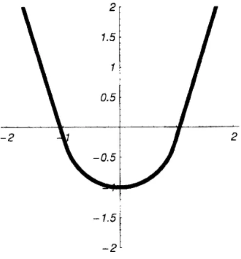
$(\mathrm{i}.\mathrm{e}., \Psi\equiv 1)$,

Deckelnicketal $\lfloor\lceil 7$] proved that the solution

$u(x, t)$ of (1.3) _with$u_{0}(x)=|x|\tan(\theta_{0}-\pi/2)$

behaves

(7)

where

$Q(s)=\{$

$-\sqrt{a^{2}-s^{2}}$ $(|s|\leq|a|\cos\theta_{0})$_,

$-|s| \tan(\theta_{0}-\pi/2)-\frac{|a|}{\sin\theta_{0}}$ $(|s|>|a|\cos\theta_{0})$

(see Fig. 2). Since $s^{2}+Q(s)^{2}=a^{2}$ on $[-|a|\cos\theta_{0}, |a|\cos\theta_{0}]$, the solution looks like an

arc after an appropriate rescaling.

Figure 2: The graph of$Q$ with the case where $a=1$ and $\theta_{0}=\pi/10$

Next consider the anisotropic case. Set

$\hat{C_{\tau_{3}}}(\theta):=a\{\Psi’(\theta)\cos(\theta-\pi/2)+\Psi(\theta)\sin(\theta-\pi/2)\}$.

By (H2), we see that $\hat{G}_{3}’(\theta)=a(\Psi^{\prime/}+\Psi)<0$. Thus we can define

$\Theta(s):=\hat{G}_{3}^{-1}(-s)$.

For the anisotropic case we can show that the limiting profile after the rescaling is

$\overline{Q}(s)$ $:=$ $\{$ $\mathrm{s}$$\tan(\theta_{-}-\pi/2)\neq\frac{a\Psi(\theta_{-})}{\cos(\theta_{-}-\pi/2)}$ for $s\leq-\hat{G}_{3}(\theta_{-})$, $-a\Psi’(\ominus(s))\sin(\ominus(s)-\pi/2)+a\Psi(\mathrm{O}-(s))\cos(\mathrm{O}-(s)-\pi/2)$ for $-\hat{G}_{3}(\theta_{-})<s<-\hat{G}_{3}(\theta_{+})$, $s$tarl$( \theta_{+}-\pi/2)+\frac{a\Psi(\theta_{\ovalbox{\tt\small REJECT}})}{\cos(\theta_{+}-\pi/2)}$

for $s\geq-\hat{G}_{3}(\theta_{[perp]})$.

(4.1)

We can check that $(s,\overline{Q}(s))$ is aportion ofa circle on the Finsler metric. This result is

(8)

References

[1] S. Angenent and M. E. Gurtin. Multiphase _{thermomechanics} _{with intcrfacial}

structure. II. Evolution of _{an isothermal interface. Arch. Rational} _Mech. Anal,_,

108$(4):323$ 391, 1989.

[2] G. Bellettini and M. Paolini. Anisotropic motion by mean curvature irl the context

of Finsler geometry. Hokkaido Math. J., 25, 537-566, 1996.

[3] M. Benes, D. Hilhorst, and R. Weidenfeld. Anisotropic... to appear, 2004.

[4] X. Chen, Generation and propagation of interfaces for reaction-diffusion equations,

J.

_Differential

Equations, 96, ₍₁₉₉₂₎ _116-141.

[5] X. Chen, $\mathrm{E}\mathrm{x}\mathrm{i}\mathrm{s}\mathrm{t}\mathrm{e}\mathrm{n}\mathrm{c}\mathrm{e}_{j}$ uniqueness, and asymptotic stability of

traveling waves in

nonlocal evolution equations, Advances in

_Differential

Equations. 2, (1997)

125-160.

[6] M. G. Crandall, H. Ishii, and P.-L. Lions. User’s guide to viscosity solutions of

second order partial differential equations. Bull. Amer. Math. Soc. (N.S.), 27,

(1992) 1-67.

[7] K. Deckelnick, C. M. Elliott, _and _{G. Richardson, Long time} _asymptotics _{for forced}

curvature flow with applications to the motion ofa superconducting vortex,

Non-linearity 10 (1997),

655-678.

[8\rceil O. $\mathrm{L}\mathrm{e}\}^{r}$. Th\‘ese de doctorat. U\gamma \iota iversit\’e de Tours, 2001.

[9] M. E. Gurtin, Thermomechanics

_of

evolvingphase boundaries in the plane, $()\mathrm{x}\mathrm{f}\mathrm{t}\supset \mathrm{r}\mathrm{d}$

Science PubL, (1993).

[10] T. $\mathrm{A}4\mathrm{a}\mathrm{r}\mathrm{u}\mathrm{t}\mathrm{a}\mathrm{n}\mathrm{i}$, H. Ninomiya and $\mathrm{R}$

, Weidenfeld, Traveling curved fronts of

anisotropic mean curvature flows, in $pre,parati$on.

[11] H. Ninomiya and M. Taniguchi, Traveling curved fronts of a mean curvature flow

with constant driving force, in ”Free boundary problems: theory and $appl\dot{\iota}cation.s.$,

$I$’ GAKUTO Internal Ser. Math. Sci Appl 13 (2000), 206-221.

[12] H. Ninomiya and M. Taniguchi, Stability oftraveling curved fronts in a curvature

flow with driving force, Methods and Application

_of

Analysis, 8 (2001), 429 450.

[13] _{H. Ninomiya and M. Taniguchi, Existence} _and global stability $()\mathrm{f}$traveling (.urved

fronts in the Allen-Cahn equations, to appear in Journal

_of

_Differential

Equations.

[14] H. Ninomiya and R. Weidenfeld, in preparation.

[15] J. E. Taylor and J. W. Cahn, Diffuseinterfaceswithsharp cornersand facets: Phase