Is Inflation Fiscally Determined?
著者
Bazzaoui Lamia
journal or
publication title
TERG Discussion Papers
number
411
page range
1-78
year
2019-07-31
TOHOKU ECONOMICS RESEARCH GROUP
Discussion Paper
Discussion Paper No.411 Is Inflation Fiscally Determined?
Lamia Bazzaoui
2019 / 07 / 31
GRADUATE SCHOOL OF ECONOMICS AND MANAGEMENT TOHOKU UNIVERSITY 27-1 KAWAUCHI, AOBA-KU, SENDAI,
Is Inflation Fiscally Determined?
*
Lamia Bazzaoui
July 31, 2019
Abstract
The aim of the present paper is to study the relationship between fiscal variables and the inflation rate for a sample of countries, over the period 1960-2017, based on a linearized equation derived from a households ’budget constraint. This equation links the inflation rate to both fiscal and monetary policy, in addition to the growth rate. We follow the same approach as Cochrane (2019a) and analyze the impact of shocks to these three variables. Impacts from fiscal and monetary policy to the inflation rate are then decomposed between different monetary policy regimes and fiscal space categories. Results indicate that the short-term interest rate is the most significant determinant of inflation. Fiscal policy also affects the inflation rate negatively through the fiscal balance, but this effect is not robust across all mon-etary policy frameworks (this relation only holds in unstructured or loosely structured discretionary monetary policy regimes). The vari-able of fiscal space on the other hand proves to be an important factor as inflation appears to be more sensitive to both fiscal and monetary policy when fiscal space is limited. Finally, we also find that, as pre-dicted by Sargent & Wallace (1981), fiscal policy can cause inflation only when the growth rate is lower than the interest rate.
Key words: Inflation, fiscal, monetary policy, public debt, Panel VAR GMM
*We gratefully acknowledge helpful comments by Prof. Jun Nagayasu (Tohoku
Univer-sity), Professors Shin-Ichi Nishiyama (Kobe UniverUniver-sity), Ryuzo Miyao (Tokyo UniverUniver-sity), Tsutomu Miyagawa (Gakushuin University), Ad Van Riet (United Nations University), Jaimie W. Lien (Chinese University of Hong Kong) and Yang Li (Nankai University). This paper also benefited from comments by seminar participants at the 5th HenU / INFER Workshop on Applied Macroeconomics, the 2019 spring meeting of the Japan Society of Monetary Economics and the WEAI 94th annual conference. We are also grateful to the Sunaga Fund for financial support.
1
Introduction
As public debt has been significantly increasing in the recent decades, en-suing macroeconomic imbalances, and more particularly the effects on the price level, have become a source of public concern. Nonetheless, fears of an inflation outbreak resulting from high indebtedness can only be justified if the existence of a relationship between inflation and fiscal policy is verified. In the prevailing literature, inflation is usually linked to monetary policy fac-tors. For example, the monetarist view suggests that inflation is the result of too much money chasing too few goods. But this view has been criti-cized as the relationship between money growth and inflation is not always empirically verified (e.g. Teles et al. (2016)). In addition, the link between inflation and the demand for money is becoming more questionable as we are moving towards electronic transactions and a moneyless economy while prices remain stable.
Among other factors that are usually considered, we also find monetary policy. Recent low levels of inflation are indeed thought to be the result of changing approaches to monetary policy, which, ever since the 1980s, takes into account a broader range of factors aside from money supply and uses other instruments in addition to open market operations. The list of nom-inal anchors has therefore been extended to include exchange rate targets, inflation targets through the long-run CPI and short-term interest rates on the short-run (based on the Fisher effect equation). The Taylor rule, as one method of inflation targeting was found to express accurately the monetary policy of several economies, even those such as the United States that have
not officially adopted an IT approach (Clarida et al. (2000)). Still, recently, this perspective has gotten challenged especially with the long-lasting zero bound episodes. Furthermore, the difficulty of some central banks to reach their inflation targets and the inability of many dynamic stochastic general equilibrium (DSGE) models to forecast the recent crisis called into question their effectiveness to provide efficient policy tools. After the financial cri-sis, there is a large body of work under way to model financial frictions and include the zero lower bound (ZLB) within the baseline DSGE framework (Gust et al. (2017)).
Fiscal determinacy of the price level, on the other hand, has not always been successfully demonstrated. The first pioneering theoretical contribution in this respect is Sargent & Wallace (1981). These authors stressed the fact that governments running persistent deficits should sooner or later have to finance those deficits through money creation (seigniorage), thus producing higher inflation. This research paved the way for several works, such as those on the fiscal theory of monetary policy. Although this theory does not exclude the impact of monetary variables, it also posits that, if future surpluses fail to adjust to growing public debt (through more taxes or less expenditures), then the price level must jump to ensure satisfaction of the present value government debt equation. Empirical work, however, has had little success in uncovering a strong and statistically significant connection between fiscal policy and inflation.
The aim of this paper is to study the link between fiscal variables and the inflation rate for a sample of 46 countries, over the period 1960-2017, based on a linearized equation derived from a household’s budget constraint. This
equation links the inflation rate to both fiscal and monetary policy variables, in addition to the growth rate. We follow the same approach as Cochrane (2019a) and analyze the impact of shocks to these three variables. Impact from fiscal and monetary policy to the inflation rate is then decomposed between different monetary policy regimes and fiscal space categories.
Results indicate that the short-term interest rate is the most significant determinant of inflation. Fiscal policy also affects the inflation rate nega-tively through the fiscal balance, but this relation is not robust across all monetary policy regimes. The variable of fiscal space also proves to be an important factor as inflation appears to be more easily affected by both fiscal and monetary policy when fiscal space is small. Finally, we also find that, as predicted by Sargent & Wallace (1981), fiscal policy can cause inflation only when the growth rate is lower than the interest rate.
2
Literature review
2.1
Sargent & Wallace (1981)
The first pionnering contribution that established a link between fiscal policy and the price level is that of Sargent & Wallace (1981). These authors de-rived fiscal determinacy of prices from the government intertemporal budget constraint, expressed as follows:
with Gtbeing government expenditures on goods, services, and transfers and
it−1Bt−1 expressing interest payments on the total outstanding debt, Tt the
tax revenues, Bt− Bt−1 new issues of interest-bearing debt.
This equation shows that government expenditures can be funded by either taxes, new issued debt, or by printing new currency (expressed by the change in outstanding stock of non-interest bearing debt Ht− Ht−1). Based
on this relation, Sargent & Wallace (1981) provided the following expression of real government deficits Dt as
Dt= (Ht− Ht−1)/pt+ (Bt− Bt−1)/(1 + Rt−1) (2)
with pt the price level at t, and Rt−1 the real interest rate on government
bonds between two periods.
From this relation, they derived an expression of the inflation rate de-pending on the stock of interest bearing government debt per capita. This model is based on the assumption that fiscal policy dominates monetary pol-icy. That is, the fiscal authority independently sets its budget, announcing current and future deficits and surpluses. And the amount of revenue to raise is then determined based on those decisions. The monetary authority then finances with seignorage any discrepancy between the revenue demanded by the fiscal authority and the amount of bonds that can be sold to the public. Also, using the assumption that interest rates on bonds are greater than the economy's growth rate, authors concluded the following: the real stock of bonds will keep growing faster than the size of the economy. But since the demand for bonds places an upper limit on the stock of bonds, eventually
financing of principal and interest will be made through seignorage. In other words, decisions of the fiscal authority can induce more money printing and therefore inflation.
2.2
The government debt valuation equation
As a basis of the fiscal determinacy of prices, the following government debt valuation equation has been suggested by several authors (Sims (1994), Woodford (1994), Woodford (1995),Woodford (1998)).
Nominal government debt/price level =Expected present value of future pri-mary surpluses Or Bt−1 pt = ∞ X j=0 Et(mt,t+jst+j) (3)
with Bt−1= one-period nominal debt issued at t − 1 due at t, pt= price level,
st=real primary government surplus including seignorage, mt,t+j= a discount
factor.
In some cases, this equation has been interpreted as an equilibrium con-dition resulting from the intertemporal government budget constraint. But in other contributions, such as Cochrane (1998, 2005), this relation has been derived as a valuation equation for government bonds seen as securities. The underlying idea is that nominal debt, including the monetary base, is a claim to future government primary surpluses (in the same way a stock is a claim to future earnings). As underlined in Cochrane (2018), bonds prices are de-termined by the market depending on bond yields and on future streams of expected primary surpluses.
2.3
Models of the fiscal theory of monetary policy
In a more recent contribution, Cochrane (2019a) provided a study of the fiscal roots of inflation based on a linearized identity, showing that unexpected inflation less the unexpected nominal return on government bonds must equal the innovation in the sum of futures surplus to GDP less the sum of future real bond returns. The derived linearized flow identity is as follows
vt+ rt+1n − πt+1− gt+1= st+1+ vt+1 (4)
vt represents the market value of debt, rtn nominal returns on the portfolio
of government debt, πt the inflation rate, gt GDP growth, st real primary
surplus, rn
t − πt− gtthe discount rate for the right-hand side terms. Variables
are expressed in log terms.
The main results of structural shocks analysis are as follows. The disin-flation of a recession shock corresponds entirely to a decline in discount rates leading to higher debt. A positive monetary policy shock (moving interest rates but not PV of future primary surpluses) is super-Fisherian and raises inflation immediately. A negative fiscal shock (moving PV of future primary surpluses but not interest rates) induces a protracted inflation. Quoting the author’s conclusion (p. 31) regarding effects of a negative shock to primary surpluses:
A fiscal shock sets off a protracted inflation. Three quarters of the fiscal shock is transmitted to future inflation via a decline in
long-term bond prices.
Finally, Sims (2011) suggested a comprehensive theoretical framework, based on the idea that even in an active fiscal, passive monetary policy equi-librium, monetary variables still have a powerful effect on both output and inflation. This model includes assumptions of a long-term public debt, an interest rate target rising with inflation and output, and fiscal surpluses de-fined by output (pro-cyclical). Different versions of this model were provided: a simple flexible-price model of an endowment economy, a model with only short-term government debt and a new-keynesian style model with long-term debt and sticky prices. This latter version includes the following equations (the derivation and solution of this model are provided by Cochrane (2018)):
M onetary policy : ˙r = −γ (r − ¯ρ) + θ ˙p + ∅ ˙c + εm (5)
F isher∗ : r = ρ + ˙p (6)
IS∗ : ρ = −˙λ
λ + ¯ρ + εr (7)
Government budget constraint : ˙b = −b ˙p − b˙a
a + ab − ¯τ − τ (8) T erm structure∗ : r = a − ˙a
a (9)
P hillips curve∗ : p = β ˙¨ p − δc − εpc (10)
F iscal policy : ˙τ = w ˙c + ετ (11)
habit∗ : λ = e−σc+ ψ (¨c − ¯ρ ˙c) e−c (12) r is the nominal interest rate, ρ is the real interest rate, with steady state
and consumer discount rate ¯ρ, p is the log of the price level, c is consumption which equals output, λ is the marginal utility of consumption, b is the real market value of government debt (consisting of nominal perpetuities), a is the consol rate, τ is the primary surplus, ¯τ is a parameter, it represents the value of τ around which the model was linearized. Starred equations are forward-looking, which implies that shocks are white noise with no effect.
Based on this framework, the requirement that the real value of debt matches the present value of future primary surpluses can be met through jumps in the interest rates which changes the value of outstanding debt even in the case of sticky prices. Also, the author underlines the fact that effective monetary measures to reduce inflation lead to a drop of inflation at first and then produce exactly the opposite effect after a delay. This has been dubbed “the stepping on a rake“ phenomenon. Evidence was shown through impulse response functions. On the other hand however, an expansionary fiscal shock creates a boom in consumption and an upward unanticipated jump in the inflation rate.
Cochrane (2018) provided the following explanation to reaction of prices in this model: if the market value of bond prices decreases, following an in-crease in interest rates for example (due to monetary policy action), without a change in future surpluses, the price level must adjust. If prices do not adjust, then the real value of government debt to investors would be greater than its real market value. People will therefore try to buy more government debt and thus less goods and services which will lead to lower aggregate de-mand and thereby lower prices. The same deflationary force would follow in case of an increase of the present value of real future primary surpluses.
A more recent trend in the literature establishes a link between the level of public indebtedness and the fiscal space.
2.4
Public debt and fiscal space
The most widely used definition of fiscal space is the one provided by Heller (2005) and according to which fiscal space reflects the availability of budgetary room that allows a government to provide resources for a desired purpose without any prejudice to the sustainability of a government’s financial posi-tion. These resources can be accessed through specific fiscal policy measures, but also through various other channels such as borrowing, seignorage, grants or institutional reforms. Therefore, the definition of fiscal space is closely linked to a government’s fiscal sustainability and its potential to expand its financing capacity. In other words, the availability of fiscal space implies that a government is able to find resources to finance a desired expenditures program and to service its debt obligations.
Even though fiscal space refers to the same concept in most macroeco-nomic policy discussions, concrete measures of fiscal space used in the empir-ical literature differ significantly across the existing studies. One commonly used approach is the ’fiscal gap’ approach. It is based on the idea of estimat-ing the difference between a given level of public debt or the fiscal balance and a benchmark level considered as the sustainability level (Ostry et al. (2010), Ghosh et al. (2013))
The sustainable debt level d∗ is estimated in different ways. In some cases, it is considered as the mean level of debt for a given group of countries. Another approach for estimating d∗is the signal approach (the debt threshold that maximizes the ratio of percentage of correctly classified debt crises in total crises observations divided by the percentage of falsely classified crises in non-crises observations), suggested by Kaminsky et al. (1998). In some other cases, a forward-looking approach is used by computing the present value of future primary balances (International Monetary Fund (2012)), as in the valuation equation. Such a methodology has been popularized by Bohn (1998, 2007, 2008). In these studies, fiscal solvency is considered to be fulfilled when the primary balance reacts positively to an increase in public debt. This approach derives the relationship between debt and the primary balance from the intertemporal government budget constraint:
dt+1− dt= (rt− gt) dt− pst+1
where dt is one-period debt (as a share of GDP) at the end of the period, g is
the growth rate of real GDP which is assumed to be exogenous and constant, pst is the primary balance (in percent of GDP), and rt is the real interest
rate on debt contracted in period t and due in period (t+1). Based on this relation, the maximum sustainable level of the primary balance is determined depending on the different interest rate-growth rate (rt− gt) which differs
across countries.
Some of the criticisms expressed against Bohn’s methodology is that it does not take into account the endogenous relation between debt and the
interest rate, and it also does not rule out the possibility of an infinitely increasing debt. These issues are addressed in the models suggested by Os-try et al. (2010) and Ghosh et al. (2013) based on which response of the primary balance to public debt is nonlinear and the interest payment sched-ule depends on the debt level. In these models, the interest rate becomes infinite beyond the debt limit as there is no finite rate that would compen-sate creditors for the probability of default (which becomes equal to unity). The level of the primary balance reaction function is determined by country-specific factors (including trade openness, inflation, current and future age dependency, commodity prices, fiscal instability, presence of fiscal rules, and international influence on fiscal behavior).
The use of the intertemporal government budget constraint is also found in contributions such as Buiter (1985), Buiter et al. (1993), Blanchard (1990), Auerbach & Gale (2011) where an index of fiscal sustainability is derived based on projections on future balances, also based on the macroeconomic outlook and forecasts of the discount rate. In addition, using the fiscal gap approach, some publications by the IMF, such as the Fiscal Monitor, present a measure of fiscal adjustment by country (inverse of fiscal space), defined as the distance between the 2011 cyclically adjusted primary balance and that needed to reduce the general government debt ratio to a sustainable level.1
Finally, Aizenman & Jinjarak (2010) suggested an alternative fiscal space measure called de facto fiscal space, defined as the inverse of the number of
1Equivalent to 60 percent of GDP in advanced economies and to 40 percent of GDP
in emerging economies and low-income countries by 2030 (or to 2012 levels, if these were lower than the 60 and 40 percent benchmarks). For Japan, a net debt target of 80 percent of GDP is assumed.
tax-years needed to repay the debt. This ratio requires the estimation of the de facto tax base corresponding to the realized tax collection averaged across multiple years to smooth for business cycle fluctuations. In Aizenman et al. (2019), this fiscal space measure is used to examine fiscal cyclicality across a large sample of countries. Authors find that lower fiscal space coincides with government-spending procyclicality.
2.5
Empirical literature on the fiscal determinacy of
prices
Results of the existing studies about the fiscal policy-inflation relationship are mitigated. No conclusive evidence was obtained so far in favor of, nor against the existence of a fiscal determinacy of the price level. Table 1 sum-marizes some of these contributions. Some of these studies focused on the link between fiscal deficits and inflation, while others examined the relationship between fiscal surpluses and public debt or used a different approach.
For example, Catao & Terrones (2005) examined the existence of a re-lationship between inflation and fiscal deficits through a study covering 107 countries over 1960 to 2001, based on a dynamic non-linear model, but could only verify it for the high-inflation, developing economies. Fischer et al. (2002) also conducted a study on 94 economies, and concluded that fiscal deficits are the main drivers of high inflation, but only in high-inflation coun-tries. More specifically, they found out that a reduction in the fiscal balance by 1 percent of GDP, leads to an increase in the inflation rate by 4.2 percent in this specific group.
Bohn (1998) followed a different approach. He examined the U.S. deficit and debt processes and showed that the primary surplus responds positively to the debt to GDP ratio. Since evidence was found that the surplus does adjust, and in a sufficient manner to ensure that the intertemporal govern-ment budget constraint holds, the author concluded that the fiscal authority acts in a ricardian fashion. As stated above, this methodology also implies that a positive adjustment of primary surpluses to public debt indicates the availability of sufficient fiscal space.
Following Bohn's approach, Bajo-Rubio et al. (2009) used cointegration analysis between the primary surplus to GDP variable and the public debt to GDP ratio, complemented with Granger causality tests for a sample of 11 EU countries, over the period 1970-2005. The authors concluded that there was no clear evidence supporting the fiscal theory of the price level (FTPL), as primary surpluses responded positively to the debt to GDP ratio in almost all cases. Other studies, such as Canzoneri et al. (2001), Creel & Le Bihan (2006), reached the same conclusion. Conversely, some others (for example Favero & Monacelli (2005)) showed the presence of alternated ricardian and non-ricardian regimes.
There are also empirical studies that led to the validation of the FTPL. For instance, Loyo (1999) argued that Brazilian policy in the late 1970s and early 1980s was non-Ricardian and that the FTPL provides a persuasive explanation for Brazil's high inflation during that time. Tanner & Ramos (2003) found evidence of fiscal dominance for the case of Brazil for some important periods. Fan et al. (2013) investigated whether the FTPL can explain UK inflation in the 1970s. They found evidence that fiscal policy
was non-Ricardian and money growth entirely endogenous in this period. Their conclusion was that government expenditures were the only driving force for inflation and therefore that the 1970s inflation outburst resulted from an increased level of expenditures, unmatched in the previous decades. Most of these previous studies used the government’s intertemporal bud-get constraint as a foundation for the choice of variables. For instance, Bohn (1998) and Canzoneri et al. (2001) based their verifications on the relation-ship between public debt and the primary balances, using the assumption that an adjustment between these two variables would be an indication of a ricardian regime. In these studies, a regression model between these two variables served as a basis. However, as pointed out by Bajo-Rubio et al. (2009), the presence of such a relationship is compatible with both a MD and a FD regime, since a price increase could be responsible for a fall in the public debt ratio, indirectly by causing a decrease in the expected value of future surpluses. To address this issue, the author included Granger causality tests between primary surpluses and debt, in addition to the cointegration analysis.
Another way to account for effects of the price level would be using the government debt valuation equation. This is a more direct way of verifying the fiscal theory of the price level. However it would be difficult to draw conclusions based on this method, for many reasons: first, the variable of the present value of future primary surpluses would be hard to measure and to analyze.2 Second, the choice of the discount rate would have a significant
2Judgment could be biased by business cycle fluctuations as primary surpluses are likely
impact on the obtained results. And in addition, as indicated by Cochrane (2019b), a change in inflation could be the reflection of a change in the dis-count rate, not a movement in fiscal variables. Finally, another critique to previous approaches in the empirical literature is that most of them exam-ined fiscal variables exclusively without taking into account interactions with monetary policy, in a single model,3 as in Sims (2011). In this respect, the
approach used by Cochrane (2019a) is innovative in the sense that it uses one single linearized relation to examine links between inflation and both fiscal and monetary variables, in addition to the business cycle (based on US data).
In the present paper, we use an approach similar to Cochrane (2019a), but with a different derivation of the linear relation of inflation, using a consumer’s budget constraint, and variables expressed in real terms. Also, as opposed to the methodology used in that study, we do not derive the value of primary surpluses from the linear identity but instead use actual data to construct a panel VAR Model. We then examine effects of a fiscal policy shock, a monetary policy shock and a recessionary shock on our variables, for a sample of 46 countries over the period 1960-2017. Finally, we further extend our study by examining how the choice of a monetary policy regime, and how the level of fiscal space affect the links between our variables.
3
Theoretical model
Based on a theoretical framework similar to Woodford (1994), we use the following consumer’s budget constraint (in nominal terms):
ptct+ Bt− Bt−1= Rt−1Bt−1+ ptyt− Tt (13)
where pt is the price level, ct consumption, Bt the portfolio of assets
(as-sumed to be consisting of government bonds only), Rt the interest rate on
government bonds, yt the household’s income, and Tt the amount of taxes.
This relation states that the sum of consumption and assets purchases is equal to the sum of interest earnings on assets held from the previous period in addition to income less tax payment. Assuming that the economy’s global income yt=gt+ ctwith gt being government expenditures, we get
Bt− Bt−1− Rt−1Bt−1= Gt− Tt (14)
For a being the % change of the value of debt, we have Bt= (1 + a) Bt−1.
Therefore
Bt−1(a − Rt−1) = Gt− Tt= −P St (15)
Because the change in public debt also depends on government bonds yields, we suppose that the following expression is valid (for a given coefficient k):
a = kRt−1 Therefore Bt−1 = P St Rt−1(1 − k) (16)
Rescaling by real GDP yt, and with θt being GDP growth, we have Bt−1 yt−1θt = P St ytRt−1(1 − k) (17)
For Byt−1 representing the term Bt−1 rescaled by GDP and P Syt the term
P St rescaled by GDP, we get
Byt−1=
θtP Syt
Rt−1(1 − k)
(18)
Because the term representing bond yields Rt−1 depends on debt maturity,
if we suppose that there is only one category of bonds with maturity n, the term structure equation implies that: Rn
t = itit+1it+2. . . it+n−1 (for it the
annualized short term interest rate). Replacing in Equation (18) Byt−1= θtP Syt Qn j=tij1/n(1 − k) (19) Dividing by pt Byt−1 pt = Qn θt j=tij1/n(1 − k) P Syt pt (20)
With the output-adjusted real primary surplus being psyt=P Sptyt and inflation
corresponding to πt= ppt−1t we get Byt−1 πtpt−1 = Qn θtpsyt j=tij 1/n(1 − k) (21)
Considering that real debt over GDP byt−1= Byt−1 pt Then byt−1 πt = θtpsyt Qn j=tij 1/n(1 − k) (22) Taking logs
log (byt−1) − log (πt) = log(θt) + log (psyt) −
1 nlog n Y j=t ij ! − log (1 − k) (23)
In this equation, the level of inflation appears to be affected by both fiscal and monetary policy, in addition to growth. As in Cochrane (2019a), we expect a positive relationship between inflation and public debt, and a negative relationship with the fiscal balance. According to the author’s model and empirical findings, higher fiscal deficits should indeed lead to higher inflation. Also response of inflation to the interest rate is assumed to be positive, consistent with the neo-Fisherian view and conclusions in Sims (2011) and Cochrane (2018).
Finally, we expect a negative relationship between inflation and the GDP growth rate. This result contradicts the conventional view based on the keynesian and neo-keynesian framework and according to which this relation should be positive (AD-AS model, Phillips Curve). However, our assumption is consistent with the findings of several empirical studies and theoretical frameworks. First, the model developed by Stockman (1981) established that an increase in the inflation rate results in a lower steady state level of output, by reducing the purchasing power of money balances, and thereby the demand for goods and for capital (assuming that a part of investment
projects is financed through cash). Second, most money and endogenous growth models concluded that the inflation rate reduces both the return on capital and the growth rate on the long-run (see Aratawari et al. (2016), Haslag (1998), Vaona (2012)).
Empirically, several studies revealed an overall negative effect of inflation on growth, and many of them also detected the presence of a non-linearity in this relationship. Kormendi & Meguire (1985) was among the first con-tributions to shift common beliefs about this relationship (from a positive to a negative one), based on a study using data for 47 countries over the period 1950-1977. Fischer (1993) found that inflation negatively affects out-put growth through the channels of investment and productivity growth. These effects were found to be particularly prominent for a high inflation rate. De Gregorio (1992) also found a negative relationship between the two variables, using pooled cross-section time series regressions for a large set of countries.
Gomme (1993), applied Lucas Jr (1988)’s endogenous growth framework combined with a cash-in-advance exchange technology. The conclusion of the paper is that a rise an inflation reduces the marginal value of the last unit of consumption of a given period. And because this value is equivalent to the cost of the last unit of work, people are induced to work less. Reduced labor results in a slower rate of capital accumulation.
Barro et al. (1996) found that a 10 percentage point increase in inflation results in a 0.2 to 0.3 percentage points reduction in GDP growth (for a dataset of over 100 countries). This relationship was however obtained only after high inflation cases were included in the sample (above 20%). Similarly,
based on a dataset of 145 countries over the period 1960-1996, and using a multivariate panel regression analysis along with numerous robustness checks, Ghosh & Phillips (1998) found a negative and statistically significant relation between inflation and growth. Authors noted that on average, a rise of inflation from 10% to 20% reduces growth by 0.3%-0.4%, and from 20% to 40% by 0.8%. Finally, Andres & Hernando (1997) found a significant negative effect of inflation on economic growth. They also found that there exists a nonlinear relationship. Their main policy message stated that reducing inflation by 1 percent could raise output by between 0.5 and 2.5 percent.
4
Variables of study and general overview of
data
This study is conducted on a sample of 46 countries (Table 2), for a period ranging from 1960 to 2017. We use yearly data from several sources for the variables of study specified in the model.
4.1
Variables of study
Because log (1 + x) ≈ x for small values of x, in some cases, variables were considered at level:
Level of Primary Balance/GDP (%): data for primary balances are re-trieved from the dataset of Mauro et al. (2013). Missing data are com-pleted from various databases such as the OECD, the World Bank and the website http://moxlad-staging.herokuapp.com/home/es for Latin
American economies.
Log of public debt to GDP: we use the underlying dataset of the paper Mauro et al. (2013). Missing data are then completed from various sources such as the website ”tradingeconomics.com” and the Reinhart & Rogoff (2009) database.
GDP growth (%): data of GDP per capita are extracted from the World Bank database
Short term interest rates: data are collected from several sources, more specifically from the IFS, Eurostat, the OECD database and in some cases from central banks’ websites. For very large values, log(1+i) is used.
Inflation rate: data are calculated from the Consumer’s Price Index (with 2010 as the base year), taken from the World Bank database. Missing data are completed based on the Reinhart & Rogoff (2009) database. For double-digit values, log(1+inflation) is used instead.
4.2
General overview of data
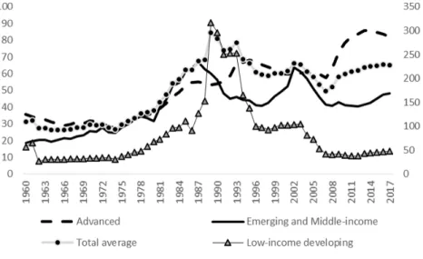
Yearly evolution of data shows that the level of indebtedness has overall been increasing over the recent years. By revenue groups (using the IMF classification), economies affected the most by this increase are advanced economies (see Figure 1); whereas the most extreme levels are observed for low-income developing economies in the 1980s (scaled on the right axis). Both developing and emerging economies have been deleveraging in the recent
decade. All sample countries suffered from increasing budget deficits after the 2007 crisis (Figure 2). But advanced economies have on average been able to reduce those deficits after 2016.
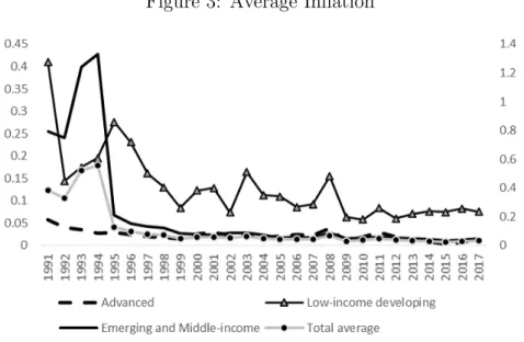
Inflation levels became very low for all countries after 1995 (see Figure 3, emerging economies and total average are modeled on right axis). The most extreme levels have been observed in the 1970s hyperinflation episode, espe-cially for advanced economies. In emerging economies, the maximum level of inflation is observed for the year 1990 due to very high values noted for Argentina, Brazil and Peru. At the same time, public debt to GDP reached its highest level in the 1980s. However, in the recent decades, the level of Public debt to GDP is lower than the high peaks of the 1980s or the year 2002 (Argentina’s debt crisis). Regarding developing economies, excessively high levels of debt accompanied by high inflation were observed in the 1980s; whereas in the recent years, the levels of both public debt to GDP and infla-tion are relatively low.
Correlation coefficients between the five main variables of study for the whole sample is provided in Table 3. The highest coefficient is the correlation between interest rates and inflation, with a positive sign (+45%). On the other hand, correlation with the fiscal variables is very weak, negative with the fiscal balance and positive in the case of public debt. Finally, GDP growth does not appear to be strongly correlated with any of the variables of study. The highest coefficient is -17% with the variable of public debt over GDP.
Using the model described in the previous section, forecast error vari-ance decomposition of inflation is generated using Cholesky decomposition
based on an active fiscal policy/passive monetary policy setting. Therefore, the following ordering of the variables is adopted: the primary balance over GDP (most exogenous), public debt over GDP, GDP growth, short-term in-terest rates, Inflation. Results clearly indicate that a significant share of the forecast error variance of inflation can be explained by exogenous shocks to the interest rates (between 10% at the beginning and 21% at the end of the observation period) or past inflation (88% at period 1) (see Figure 4). The share of shocks to the primary balance, although not null, is very small (varies between 1.4% and 2.7%). Therefore fiscal policy does affect inflation but not to the same extent as monetary policy. The impact of public debt on inflation is almost absent (around 0.6%).
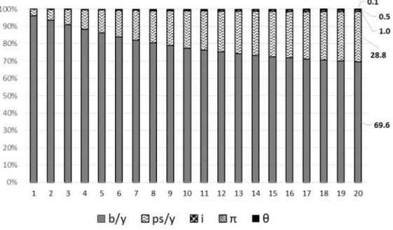
Using the same model to generate forecast error variance decomposition of public debt (Figure 5), we also do not find evidence of a contribution of inflation to public debt (limited to 0.5%). Public debt is significantly af-fected by past debt (around 70%) and a growing contribution of the primary balance shocks (as expected) (reaching 28.8%), but other variables are in-significant. Interestingly, the variance decomposition of a one-period lagged public debt shows a more significant contribution of growth (close to 10% at the 20th period).
4.3
Monetary policy frameworks
As stated in the introduction, some analysts attribute the generalized low level of inflation to a major change in monetary policy frameworks. This shift
in monetary policy thinking by setting up rules or targets (money, credit, ex-change rate, interest rates, and inflation) aimed at addressing the dynamic inconsistency issue (Kydland & Prescott (1977), Calvo (1978)). Dynamic in-consistency refers to changes in the decisions of monetary authorities and the absence of commitment to a single optimal policy. Especially when output is below the optimal level, monetary authorities have an incentive in moving away from an announced target in order to generate a “surprise“ inflation and thereby a short-term increase in growth. So it is usually based on the underlying idea that the relationship between inflation and GDP growth is positive.
A consensus in this literature is that commitment is a better policy be-cause it generates lower average inflation in the long run (Barro & Gordon (1983), Rogoff (1985)). The gains from commitment are a direct consequence of the role that expectations play in shaping economic conditions. More specifically, Inflation Targeting regimes are thought to have contributed to reduce inflation levels and increase monetary policy credibility.
To verify this assumption we use the classification provided by Cobham (2018) for our sample. The author defines a monetary policy framework as a combination of objectives, constraints and conventions for monetary au-thorities. Constraints and conventions include “rules or disciplines to which authorities are subject (voluntarily or involuntarily), the nature of the fi-nancial and monetary markets and institutions, the understandings of key macroeconomic relationships, and the political environment“. Among the criteria used to distinguish between different frameworks is the verification of whether monetary authorities publish targets for some objective and whether
such targets exist for monetary aggregates, exchange rates, inflation or other variables. Based on this definition and other additional criteria, the author identifies 32 different categories, aggregated into 9 broad categories based on target variables.
Direct controls: multiple exchange rates and/or controls on direct lend-ing, interest rates, etc
Fixed exchange rates: exchange rate fixed by intervention, some or no monetary instruments in use or pure currency board (domestic currency 100% backed by foreign currency, no monetary instruments in use) Exchange rate target
Monetary target Inflation target
Mixed targets: monetary targets and exchange rate fixes or targets, monetary dominant or use of three full targets (or fixes) (money, ER and IT), whichever dominant
Unstructured, loosely structured discretion: ineffective set of instru-ments and incoherent mix of objectives
Well structured discretion
No national framework: this category encompasses cases where a dif-ferent sovereign currency is used (such as dollarization) in addition to membership in a currency union (euro)
Some of these categories are not represented in our sample and Cobham (2018)’s database does not include some of our sample countries (we aggre-gated them within the ”No national framework” category).
Examining the data (Figure 6), we can see that the IT regime has spread significantly after the 1990s, while monetary target frameworks disappeared and exchange rate targets and discretionary regimes became less frequent. Data shows that levels of inflation are low in all cases in the recent decades. However, during the 1980s, exceptionally high levels of inflation are noted for mixed targets regimes (France, Germany and Italy). If there is no fiscal dom-inance in our sample then the choice of monetary policy frameworks should affect how inflation reacts to fiscal variables. More specifically, if monetary policy is the major driver of inflation, we expect that the inflation-fiscal pol-icy relation will be weakened in commitment monetary polpol-icy regimes, and more particularly inflation targeting.
4.4
Fiscal space
Observing levels of debt alone is not sufficient to draw conclusions about a government’s solvency. Therefore we introduce the notion of fiscal space in our analysis to account for a government’s capacity to repay contracted debt. We use a definition that is closer to that of Aizenman & Jinjarak (2010). We first calculate the ratio of public debt divided by total government revenues. This measure reflects the number of years of revenue needed to repay the outstanding of public debt at a given date. Fiscal space is then defined as the inverse of that ratio. The most recent available value (2016), the average
and some descriptive statistics of the calculated measure are given for all sample countries in Table 4.4
As shown on Figure 7, countries with the lowest fiscal space in the 1980s are Colombia and Nicaragua. In 2016, Japan has the lowest fiscal space with the greatest number of years required to repay the debt (see Figure 8). Simple observation of those two figures does not show an obvious link between the fiscal balance and fiscal space, since both groups of countries running substantial budget deficits and those with high surpluses can have either low or high fiscal space. This implies that fiscal policy does not necessarily depend on this ratio.
However, correlation coefficients appear to be significant in many coun-tries (Table 5), even though the correlation sign varies (it is negative in cases like Japan, Australia, Brazil and the USA, and positive in some other cases, such as Belgium, Mexico and Pakistan, etc). After the 2007 crisis, the fiscal space measure has worsened for advanced economies in particular (for exam-ple Japan, from 3.4 to 6.9 or the USA, from 1.8 to 2.9), reflecting the use of fiscal stimulus after the recession. On the other hand, emerging and de-veloping economies, which suffered from a deteriorating fiscal stance during the 1980s debt crisis, have had a better fiscal space indicator over the last decade.
4To reduce gaps in data, missing values have been filled using the closest available
5
Results and discussion
We estimate the following VAR model
zt = ∅1zt−1+ . . . + ∅jzt−j+ wt (24) where zt = psyt byt θt it πt ∅j = ∅j11 ∅j12 ∅j13 ∅j14 ∅j15 ∅j21 ∅j22 ∅j23 ∅j24 ∅j25 ∅j31 ∅j32 ∅j33 ∅j34 ∅j35 ∅j41 ∅j42 ∅j43 ∅j44 ∅j45 ∅j51 ∅j52 ∅j53 ∅j54 ∅j55 and wt = v1t v2t v3t v4t v5t
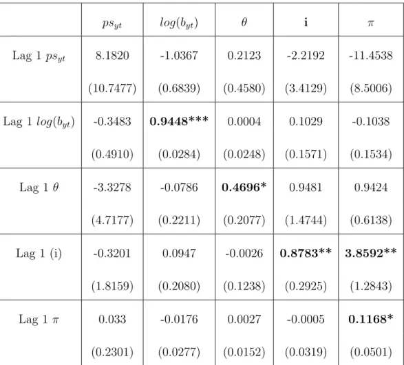
The estimation is made using the methodology suggested by Sigmund & Ferstl (2017) for panel VAR GMM (details provided in Appendices 1 and 2), and after applying forward orthogonal transformation to the variables of study (see Appendix 3). The methodology of Sigmund & Ferstl (2017) is useful to eliminate the Nickell Bias (Nickell (1981)), according to which the correlation between error terms and regressors present in panel VAR OLS estimations leads to inconsistent estimators. The resulting model is shown on Table 6).
Results indicate that public debt is persistent with a significant autore-gressive coefficient. The variables of growth, interest rate and inflation also have a significant own coefficient. The inflation equation shows that the only significant variable in determining inflation is the interest rate, with a positive and high coefficient. Fiscal variables’ coefficients are negative but
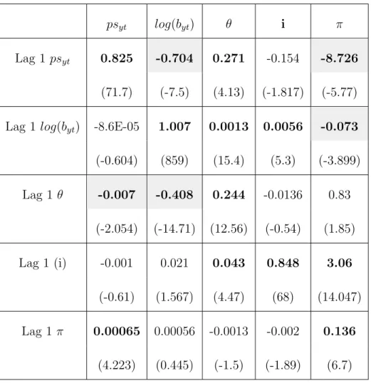
not statistically significant. OLS estimation, on the other hand (Table 7), shows that both fiscal policy and monetary policy variables significantly af-fect the variables of study. Also, the primary balance reacts positively to debt (consistent with our expectations), while debt is affected negatively by the primary balance (as cumulating budget deficits lead to a growing debt). The variable of growth has a negative effect on both the fiscal balance and public debt.
5.1
Inflation’s interdependence with the variables of
study
Using generalized impulse response functions to analyze the impact on infla-tion of a one-standard deviainfla-tion innovainfla-tion in all variables (Figure 9), we note a positive and very significant response to interest rates (a 1 to 1 response). A positive shock in the primary balance also induces a positive response of inflation (higher surplus implies higher inflation), but of a smaller magnitude (0.3 units). These first results indicate that inflation is affected by both fiscal and monetary policy. However, response of inflation to public debt is very small and of a negative sign (less than -0.1 at period 1). Similarly, a shock to growth also leads to a very limited, negative response of inflation.
On the other hand (see Figure 10), we also observe responses of all vari-ables to a one-standard deviation innovation in inflation. We note that this shock induces a positive and very significant response in short-term interest rates (0.05 units). Public debt to GDP (in log terms) responds negatively over the long-run (but with a magnitude limited to -0.01). Responses of
other variables are very small.
5.2
Fiscal policy shock
A one standard deviation positive innovation in the primary balance (Fig-ure 11) induces a positive but poor response of growth and the interest rates (less than 0.02 units). This suggests that fiscal policy does not affect mone-tary policy. On the other hand, a significant and negative response of public debt over GDP (in log terms) is generated over the long-run (reaching -0.1 at the end of the period). However, response of the inflation rate is the most notable one. After a positive jump, inflation gets negative immediately in the second period (which is consistent with findings of the previous subsec-tion) reaching the value of -0.15. Therefore a policy that increases taxation or reduces government expenditures would eventually lead to lower future debt and lower inflation. Similarly, an expansionary fiscal policy induces the opposite effect as applying a negative shock to the primary balance leads to a positive jump in the inflation rate, suggesting that fiscal deficits are inflationary.
Nevertheless, when we split data based on monetary policy frameworks’ classification provided by Cobham (2018)(for the period 1980-2016), we find that the relationship between inflation and the fiscal balance varies across monetary policy regimes. First, the correlation coefficients, although not very high, are very different. The highest level of correlation is +23% in the case of discretionary regimes (Figure 12). Second, when we decompose
generalized impulse response functions of inflation to a fiscal shock based on monetary policy frameworks (Figure 13), we notice that the negative response of inflation is only seen in unstructured or loosely structured discretionary regimes (and with a magnitude lower than the response obtained for the whole sample), while no response is noted for other monetary policy frame-works. Mixed targets regimes do show a positive response in the long-run, but due to the small number of observations (3 countries in the 1980s), it is difficult to draw any conclusions. We find the same result when estimating a GMM model for inflation based on the different frameworks (Table 8). Inter-estingly, short-term interest rates do not appear to be statistically significant in inflation targeting and exchange rate targets regimes.
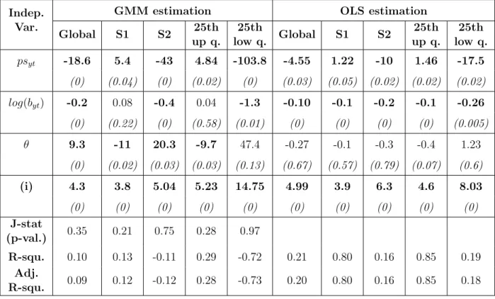
In the following step of the study, in order to see how fiscal space affects the relationship between inflation and the fiscal variables, we split our sam-ple into two fiscal space categories based on the middle quartile. S1 is the subsample of higher fiscal space countries, for which few years are needed to repay the debt and S2 is the subsample of economies with lower fiscal space, for which many years are needed to repay the debt burden. Results (Table 9) indicate that correlation between inflation and the fiscal balance is positive with higher correlation for economies with the lowest levels of fiscal space.
Using generalized impulse response functions (Figure 14), a strong posi-tive (up tp +0.6 units), then negaposi-tive (to -0.4), response of inflation to a pos-itive shock to the primary balance is noted for the S2 subsample (economies with low fiscal space) while in the case of S1, response of inflation is very weak and positive (+0.2). The implication is that countries with lower levels of fiscal space are more at risk of inflationary pressures in case of increasing
deficits. Focusing on the upper and lower 25th quartiles also corroborates this conclusion, as no response is obtained for the upper quartile (see Fig-ure 15). Decomposing impulse response functions of S2 (economies with low fiscal space) by monetary policy regime shows once again that (even for the isolated case of S2) the relationship between inflation and fiscal policy only holds for discretionary regimes (Figure 16).
Table 10 shows an estimated regression model of inflation using GMM (with lagged variables as instruments) and OLS. We can see that for sub-samples with high fiscal space, the coefficient of the fiscal balance is positive but not vey high (around 5 in the GMM specification and 1 based on OLS). In the case of subsamples with low fiscal space, that coefficient is negative, statistically significant and of a much higher magnitude (-103.8 for the 25th lower quartile in the GMM model).
Because both discretionary monetary policy regimes and low fiscal space are factors that determine the existence of a relationship between fiscal policy and inflation, we plot the number of observations by fiscal space depending on monetary policy frameworks (Figure 17). Difference between fiscal space categories in terms of number of observations for discretionary regimes is not very notable. This implies that discretionary regimes are not necessarily reflective of cases of low fiscal space. Therefore, both factors are important. Finally, focusing on the public debt variable, the correlation coefficient of inflation with public debt (Table 9) is negative in the case of S1 (meaning that higher debt for countries with enough revenues has a negative effect on inflation), and positive and significant for S2 (public debt is associated with high inflation in countries with low fiscal space). Generalized impulse
response functions show a positive response of inflation to a shock to public debt(Figure 18 and Figure 19). By fiscal space categories, this relationship appears to hold only for lower fiscal space countries.
5.3
Monetary policy shock
A positive one SD innovation in short-term interest rates induces a positive and notable response of the inflation rate, of 0.9 (Figure 20). No response is obtained for primary balances which implies that monetary policy does not affect fiscal policy. Response of other variables is very small and negative. The correlation coefficient between inflation and short-term interest rates is also positive and very important (as opposed to fiscal policy)(see Figure 21 and Table 9). The most significant values are observed for discretionary monetary targets and mixed targets regimes.
As in the previous subsection, we decompose generalized impulse response functions of inflation following monetary policy shocks using the monetary policy frameworks’ classification (Figure 22). This time, the most significant responses are those of both discretionary and exchange rate regimes. As in the previously estimated GMM model (Table 8), response of inflation to the interest rate is weaker in inflation targeting regimes.
Impulse response functions by categories of fiscal space show that the response on inflation is stronger in lower fiscal space countries (Figure 23). The same result is obtained by focusing only on the 25th upper and lower quartiles (Figure 24). This result is also corroborated by the regression model discussed previously (Table 10) where coefficient of the interest rate appears
to be much more significant in the case of countries with lower fiscal space.
5.4
Recessionary shock
In a final step, we apply a -1 unit shock to growth to see the impact of reces-sionary episode on the variables of study (Figure 25). Response of inflation (modeled on the right axis) is strong and gets negative in the second period (to -0.8), but quickly resumes back to its level (consistent with a Phillips curve as the growth level also adjusts). No response is shown for the pri-mary balance and the interest rate. Public debt responds positively over the medium-term (which is consistent with our expectations). Therefore while the relationship between debt and growth is visible, growth does not ap-pear to affect the other variables, which confirms findings of the previous subsections.
The growth rate could however affect the existence of a relationship be-tween fiscal variables and inflation. As pointed by Sargent & Wallace (1981), fiscal policy affects the price level when interest rates are greater than the growth rate, and thereby the cumulating burden of debt gradually surpasses the demand for bonds by investors. To check this assumption, we split data between observations where growth is greater than the interest rate and ob-servations with growth lower than the interest rate (for which we expect to see a stronger relationship between fiscal policy and inflation). Results (Fig-ure 26) clearly corroborate this idea as no response from inflation is obtained in the case where growth is greater than the interest rate.
5.5
Absence of fiscal dominance
Previous empirical studies, notably Bohn (1998), Bajo-Rubio et al. (2009) and Canzoneri et al. (2001), rejected fiscal determinacy of the price level and concluded that governments act in a ricardian fashion because of the presence of an adjustment of primary surpluses to changes in public debt. We also find a similar result when we examine the response of fiscal balances to a shock to public debt. And reciprocally, as in Canzoneri et al. (2001), public debt reacts negatively to a positive shock to primary balances (Figure 11). Such a finding is an indication of the absence of fiscal dominance since, as stated by Tanner & Ramos (2003), the primary surplus adjusts to limit debt growth when the regime is monetary dominant (MD), so that monetary policy can be conducted independently of fiscal financing requirements. Moreover, we are unable to obtain a strong direct relation between public debt and inflation, when considering the whole sample (see FE variance decomposition of both debt and inflation in section 4).
However, when examining the relationship between fiscal balances and inflation, we find a significant negative relationship between both variables (section 5.2). This result suggests that fiscal deficits are inflationary, as in Fan et al. (2013). Still, further analysis shows that this relation is not robust across all sample countries and periods. It only holds in cases when unstructured or loosely structured discretion is applied. In monetary regimes based on targets, our results indicate that inflation is not sensitive to fiscal policy (and is also less sensitive to other shocks).
from previous discussions on monetary policy (Kydland & Prescott (1977) and Barro & Gordon (1983)) according to which inflation’s sensitivity to shocks is reduced when central banks operate under commitment. The main justification is that such regimes require independence of monetary author-ities. Therefore, in these particular cases, governments cannot force central banks to finance their deficits by generating excess liquidity or pressure cen-tral banks to keep low interest rates in order to lower governments’ borrowing costs. In the language of Leeper (1991), fiscal policy is ’passive’ and mone-tary policy is ’active’, so that there is no fiscal dominance. As a consequence, we conclude that fiscal determinacy of the price level is only possible when central banks practice unstructured/loosely structured discretion.
6
Conclusion
In this paper, we attempted to verify the presence of a relationship between fiscal policy and inflation. We used a theoretical and analytical framework similar to the one suggested by Cochrane (2019a). This approach allowed us to examine simultaneously the links between inflation, fiscal and monetary variables, and GDP growth; in contrast to previous empirical studies which only focused on the relationship between debt and the primary balance, or between inflation and some fiscal variables.
We followed a slightly different approach than Cochrane (2019a) in de-riving the linearized identity that served as a basis for our analysis. This relation was obtained from a household’s budget constraint, using variables expressed in real terms, as opposed to the government debt valuation
equa-tion in which the variable of debt alone is expressed in nominal terms. Also, we did not attempt to compute the value of primary surpluses based on the linear identity and instead we used actual data to construct a panel VAR model.
For our sample of 46 countries, over the period 1960-2017, we found a clear and positive relation between inflation and the interest rate throughout all steps of the study (GIRF showed a 1 unit response of inflation to a 1 SD innovation in interest rates). We also found that the inflation rate was neg-atively affected by the fiscal balance, suggesting that an expansionary fiscal policy is inflationary. These findings are consistent with those of Cochrane (2019a). In Cochrane’s study (which covered US data), the relationship be-tween interest rates and inflation was also found to be strong and positive and the one between fiscal balances and inflation to be negative.
On the other hand, we could not draw conclusions about the existence of a direct link between public debt over GDP and inflation. While impulse response functions showed a positive response of inflation to increasing debt, this connection did not appear clearly in the variance decomposition analysis. We also could not find a significant impact from growth to most variables. Nevertheless, we were able to verify that, as predicted by Sargent & Wallace (1981), the relationship between fiscal policy and inflation is only present when growth is lower than the interest rate.
We then further extended our analysis by examining how the choice of a monetary policy regime, and how the level of fiscal space affect the links between our variables. Interestingly, we found out that the relationship be-tween fiscal balances and inflation only holds in cases when unstructured
or loosely structured discretion is applied. In monetary regimes based on targets, our results indicated that inflation was not sensitive to fiscal policy (and was also less sensitive to other shocks). We thereby concluded on the absence of fiscal dominance. Based on these findings, fiscal determinacy of the price level is only possible when central banks do not operate under com-mitment. The most significant implication is that running persistent deficits will not lead to unexpected higher inflation, if monetary policy is resilient and credible enough to generate well-anchored inflation expectations.
Finally, we examined how fiscal space (defined as the inverse of the num-ber of years of revenue needed to repay the outstanding of public debt at a given date) affects the relationship of inflation with fiscal and monetary policy. We found that inflation is more sensitive to variations in both the fiscal balance and the interest rate when fiscal space is low.
References
Aizenman, J. & Jinjarak, Y. (2010), De facto fiscal space and fiscal stimulus: Definition and assessment, Technical report, National Bureau of Economic Research.
Aizenman, J. & Jinjarak, Y. (2012), ‘The fiscal stimulus of 2009–2010: trade openness, fiscal space, and exchange rate adjustment’, NBER International Seminar on Macroeconomics 8(1), 301–342.
space and government-spending and tax-rate cyclicality patterns: A cross-country comparison, 1960–2016’, Journal of Macroeconomics 60, 229–252. Anderson, T. W. & Hsiao, C. (1982), ‘Formulation and estimation of dynamic
models using panel data’, Journal of Econometrics 18(1), 47–82.
Andres, J. & Hernando, I. (1997), ‘Inflation and economic growth: some evi-dence for the OECD countries’, Monetary Policy and the Inflation Process-BIS Conference Papers (4), 364–383.
Aratawari, R., Hori, T. & Mino, K. (2016), On the nonlinear relationship between inflation and growth: a theoretical exposition. Kyoto University Discussion papers.
Arellano, M. & Bond, S. (1991), ‘Some tests of specification for panel data: Monte Carlo evidence and an application to employment equations’, Re-view of Economic Studies 58(2), 277–297.
Arellano, M. & Bover, O. (1995), ‘Another look at the instrumental vari-able estimation of error-components models’, Journal of Econometrics 68(1), 29–51.
Auerbach, A. J. & Gale, W. G. (2011), Tempting Fate: The Federal Budget Outlook, Brookings Institution Washington, DC.
Auerbach, A. J., Gale, W. G. & Orszag, P. R. (2002), ‘The budget outlook and options for fiscal policy’, Available at SSRN 308562 .
and inflation in EMU: An analysis from the fiscal theory of the price level’, European Journal of Political Economy 25(4), 525–539.
Baksa, D., Benk, S. & Jakab, M. (2010), ‘Does the fiscal multiplier exist?’, EcoMod2010 .
Barro, R. J. & Gordon, D. B. (1983), ‘Rules, discretion and reputation in a model of monetary policy’, Journal of Monetary Economics 12(1), 101– 121.
Barro, R. J. et al. (1996), ‘Inflation and growth’, Review-Federal Reserve Bank of Saint Louis 78, 153–169.
Bassetto, M. & Cui, W. (2018), ‘The fiscal theory of the price level in a world of low interest rates’, Journal of Economic Dynamics and Control 89, 5–22.
Bernanke, B. S., Gertler, M. & Gilchrist, S. (1999), ‘The financial accelerator in a quantitative business cycle framework’, Handbook of Macroeconomics 1, 1341–1393.
Blanchard, O., Dell Ariccia, G. & Mauro, P. (2010), ‘Rethinking macroeco-nomic policy’, Revista de Econom´ıa Institucional 12(22), 61–82.
Blanchard, O. J. (1990), ‘Suggestions for a new set of fiscal indicators’, OECD Economics Department Working Papers .
URL: https://ideas.repec.org/p/oec/ecoaaa/79-en.html
Blundell, R. & Bond, S. (1998), ‘Initial conditions and moment restrictions in dynamic panel data models’, Journal of Econometrics 87(1), 115–143.
Bohn, H. (1998), ‘The behavior of US public debt and deficits’, Quarterly Journal of Economics 113(3), 949–963.
Bohn, H. (2007), ‘Are stationarity and cointegration restrictions really neces-sary for the intertemporal budget constraint?’, Journal of Monetary Eco-nomics 54(7), 1837–1847.
Bohn, H. (2008), ‘The sustainability of fiscal policy in the United States’, CESifo Working Paper Series: Sustainability of Public Debt (1446), 15– 49.
Buiter, W., Corsetti, G. & Roubini, N. (1993), ‘Excessive deficits: sense and nonsense in the treaty of Maastricht’, Economic Policy 8(16), 57–100. Buiter, W. H. (1985), ‘A guide to public sector debt and deficits’, Economic
policy 1(1), 13–61.
Buiter, W. H. (2017), ‘The fallacy of the fiscal theory of the price level-once more’, CEPR Discussion Paper No. DP11941 .
Calvo, G. A. (1978), ‘On the time consistency of optimal policy in a monetary economy’, Econometrica 46(6), 1411–1428.
Calvo, G. A. (1983), ‘Staggered prices in a utility-maximizing framework’, Journal of Monetary Economics 12(3), 383–398.
Canzoneri, M. B., Cumby, R. E. & Diba, B. T. (2001), ‘Is the price level determined by the needs of fiscal solvency?’, American Economic Review 91(5), 1221–1238.
Carlstrom, C. T. & Fuerst, T. S. (1997), ‘Agency costs, net worth, and busi-ness fluctuations: A computable general equilibrium analysis’, American Economic Review 87(5), 893–910.
Catao, L. A. & Terrones, M. E. (2005), ‘Fiscal deficits and inflation’, Journal of Monetary Economics 52(3), 529–554.
Clarida, R., Gali, J. & Gertler, M. (2000), ‘Monetary policy rules and macroe-conomic stability: evidence and some theory’, Quarterly journal of Eco-nomics 115(1), 147–180.
Cobham, D. (2018), ‘A comprehensive classification of monetary policy frameworks for advanced and emerging economies’, MPRA Paper avail-able at https://mpra.ub.uni-muenchen.de/id/eprint/90141 .
Cochrane, J. H. (1998), ‘A frictionless view of US inflation’, NBER Macroe-conomics Annual 13, 323–384.
Cochrane, J. H. (2005), ‘Money as stock’, Journal of Monetary Economics 52(3), 501–528.
Cochrane, J. H. (2011), ‘Understanding policy in the great recession: Some unpleasant fiscal arithmetic’, European Economic Review 55(1), 2–30. Cochrane, J. H. (2018), ‘Stepping on a rake: The fiscal theory of monetary
policy’, European Economic Review 101, 354–375.
Cochrane, J. H. (2019a), ‘The fiscal roots of inflation’, Working paper avail-able at https://faculty.chicagobooth.edu/john.cochrane/research/ .
Cochrane, J. H. (2019b), The Fiscal Theory of the Price Level, Chicago Booth.
URL: https://faculty.chicagobooth.edu/john.cochrane/research/papers/ fiscal theory book.pdf
Coenen, G., Erceg, C. J., Freedman, C., Furceri, D., Kumhof, M., Lalonde, R., Laxton, D., Lind´e, J., Mourougane, A., Muir, D. et al. (2012), ‘Ef-fects of fiscal stimulus in structural models’, American Economic Journal: Macroeconomics 4(1), 22–68.
Corsetti, G. & Mackowiak, B. (2001), ‘Nominal debt and the dynamics of currency crises’, CEPR Discussion Paper (No. 2929). Available at SSRN: https://ssrn.com/abstract=281674.
Creel, J. & Le Bihan, H. (2006), ‘Using structural balance data to test the fiscal theory of the price level: Some international evidence’, Journal of Macroeconomics 28(2), 338–360.
Daniel, B. C. (2001a), ‘A fiscal theory of currency crises’, International Eco-nomic Review 42(4), 969–988.
Daniel, B. C. (2001b), ‘The fiscal theory of the price level in an open econ-omy’, Journal of Monetary Economics 48(2), 293–308.
De Gregorio, J. (1992), ‘Economic growth in Latin America’, Journal of Development Economics 39(1), 59–84.
level-identification and testing for the UK in the 1970s’, Cardiff Economics Working Papers, Cardiff University E2013/12.
Favero, C. A. & Monacelli, T. (2005), ‘Fiscal policy rules and regime (in) stability: evidence from the US’, IGIER Working Paper .
Fischer, S. (1993), ‘The role of macroeconomic factors in growth’, Journal of monetary economics 32(3), 485–512.
Fischer, S., Sahay, R. & V´egh, C. A. (2002), ‘Modern hyper-and high infla-tions’, Journal of Economic literature 40(3), 837–880.
Friedman, M. (1968), ‘The role of monetary policy’, American Economic Review 58, 1–17.
Gal´ı, J., L´opez-Salido, J. D. & Vall´es, J. (2007), ‘Understanding the effects of government spending on consumption’, Journal of the European Economic Association 5(1), 227–270.
Ghosh, A. & Phillips, S. (1998), ‘Warning: Inflation may be harmful to your growth’, IMF Staff Papers 45(4), 672–710.
Ghosh, A. R., Kim, J. I., Mendoza, E. G., Ostry, J. D. & Qureshi, M. S. (2013), ‘Fiscal fatigue, fiscal space and debt sustainability in advanced economies’, Economic Journal 123(566), F4–F30.
Gomme, P. (1993), ‘Money and growth revisited: Measuring the costs of inflation in an endogenous growth model’, Journal of Monetary Economics 32(1), 51–77.
Gordon, R. J. (1982), Why stopping inflation may be costly: Evidence from fourteen historical episodes, in ‘Inflation: Causes and Effects’, University of Chicago Press.
Gust, C., Herbst, E., L´opez-Salido, D. & Smith, M. E. (2017), ‘The empirical implications of the interest-rate lower bound’, American Economic Review 107(7), 1971–2006.
Haslag, J. H. (1998), ‘Monetary policy, banking, and growth’, Economic Inquiry 36(3), 489–500.
Hayat, Z. (2013), ‘The pros and cons of a discretionary moetary policy strat-egy: An empirical assessment’, Available at SSRN 2270210 .
Heller, M. P. S. (2005), Understanding fiscal space, International Monetary Fund.
Holtz-Eakin, D., Newey, W. & Rosen, H. S. (1988), ‘Estimating vector au-toregressions with panel data’, Econometrica 56(6), 1371–1395.
International Monetary Fund (2012), ‘Fiscal monitor: Balancing fiscal policy risks’, World Economic and Financial Surveys .
Ismailov, S., Kakinaka, M. & Miyamoto, H. (2016), ‘Choice of inflation tar-geting: Some international evidence’, North American Journal of Eco-nomics and Finance 36, 350–369.
Jiang, Z. (2018), ‘Fiscal theory, price level, and exchange rate’, SSRN Elec-tronic Journal . http://dx.doi.org/10.2139/ssrn.3059009.
Johansen, S. (1988), ‘Statistical analysis of cointegration vectors’, Journal of Economic Dynamics and Control 12(2-3), 231–254.
Kaminsky, G., Lizondo, S. & Reinhart, C. M. (1998), ‘Leading indicators of currency crises’, IMF Staff Papers 45(1), 1–48.
King, R. G. & Plosser, C. I. (1984), ‘Money, credit, and prices in a real business cycle’, American Economic Review 74(3), 363–380.
Koop, G., Pesaran, M. H. & Potter, S. M. (1996), ‘Impulse response analysis in nonlinear multivariate models’, Journal of Econometrics 74(1), 119–147. Kormendi, R. & Meguire, P. (1985), ‘Macroeconomic determinants of growth: Cross-country evidence’, Journal of Monetary Economics 16(2), 141–163.
URL: https://EconPapers.repec.org/RePEc:eee:moneco:v:16:y:1985: i:2:p:141-163
Krugman, P. & Eggertsson, G. B. (2011), Debt, deleveraging and the liq-uidity trap, in ‘2011 Meeting Papers’, number 1166, Society for Economic Dynamics.
Kydland, F. E. & Prescott, E. C. (1977), ‘Rules rather than discretion: The inconsistency of optimal plans’, Journal of Political Economy 85(3), 473– 491.
Kydland, F. E. & Prescott, E. C. (1982), ‘Time to build and aggregate fluctuations’, Econometrica 50(6), 1345–1370.