東北大学機関リポジトリTOUR

(1)

Dominance of a dipole magnetic field under the

condition of the past Earth's interior based

on numerical simulations of the geodynamo

著者

Nishida Yuki

学位授与機関

Tohoku University

(2)

博士論文

Dominance of a dipole magnetic field under

the condition of the past Earth’s interior based

on numerical simulations of the geodynamo

（数値ダイナモシミュレーションに基づく

過去の地球内部条件下における

双極子磁場卓越性に関する研究）

(3)

博士論文

Dominance of a dipole magnetic field under

the condition of the past Earth’s interior based

on numerical simulations of the geodynamo

（数値ダイナモシミュレーションに基づく

過去の地球内部条件下における

双極子磁場卓越性に関する研究）

東北大学大学院理学研究科

地球物理学専攻

西田有輝

論文審査委員加藤雄人教授（指導教員・主査）小原隆博教授笠羽康正教授寺田直樹教授熊本篤志准教授松島政貴助教（東京工業大学）松井宏晃准上級研究員（カリフォルニア大学デービス校）

令和

2 年

(4)

Acknowledgement

Foremost, I would like to express the deepest appreciation to my supervisor,

Pro-fessor Yuto Katoh for his continuous support. His advice, comments, and

encour-agement have been a great help in my study. I would also like to express the

great appreciation to Dr. Hiroaki Matsui for his kind advice. His comments and

suggestions in weakly meeting are very helpful in my study. I would also like to

express the large appreciation to Assistant Professor Masaki Matsushima for his

suggestions. His comments at scientific conferences have advanced my study and

submitted paper. I am deeply grateful to Associate Professor Atsushi Kumamoto

and Emeritus Professor Hiroshi Oya for their fruitful advice, suggestions, and

en-couragement. I extend my deep thanks to Professors Takahiro Obara, Yasumasa

Kasaba, and Naoki Terada. Their comments in their lectures or our group’s

sem-inars gave me chances to take deep thought of my study. I would like to express

the deep gratitude to members of the group of Deep Earth Physics in Kyushu

(5)

search theme in weakly study meeting. I wish to express my special thanks to the

past and present members of the Space and Terrestrial Plasma Physics Labortory.

Assistant Professors Tomoki Kimura and Yohei Kawazura gave me new

perspec-tives in my study field. Mr. Takumi Kera helped me advancing my study in daily

discussion. Finally, I would like to express heartfelt thanks to my parents, Tetsuya

(6)

Abstract

The solid inner core of the Earth has been growing for approximately one

bil-lion years due to cooling of the Earth. The changing spherical shell geometry

of the Earth’s core is likely to influence on the geodynamo driven by convective

motions in the fluid outer core. To understand the geometry effect on the dynamo

regime through evolution of the core, we perform numerical simulations of

geody-namo with three spherical shell radius ratios: ri/ro = 0.15, 0.25, and 0.35, where

ri and ro are the inner and outer core radii, respectively. To evaluate the

mor-phology of the magnetic field, we examine two indices about dipole component

dominance: (i) fdip, dipolarity used to assess the relative strength of the dipole

field at the core surface in numerical dynamo models, and (ii) fmag fit, the ratio

of magnetic energy density for the dipole component to that extrapolated from

the magnetic power spectrum for the high degree components. We investigate the

field morphology estimated from fdipand fmag fit, and find that fmag fitis valid to

(7)

number for sustained dynamos based on both fdip and fmag fit, and find that the

range of the Rayleigh number for the dynamo characterized by the strong dipole

field becomes narrower for the smaller inner core. The fdip-dependences on the

Rayleigh number obtained for ri/ro = 0.25 and 0.35 are similar to each other,

whereas the fmag fit-dependence for ri/ro = 0.35 is found to be relatively larger

than that for ri/ro = 0.25. On the other hand, small values of fdip and fmag fit

for ri/ro = 0.15 suggest that the dynamo regime is characterized not only by

the dipolar dominance but by non-dipolar dominance. These results indicate that

changes in the spherical shell radius ratio largely influence on the dynamo regime

in numerical dynamos with the fixed temperature boundary condition.

We also perform numerical dynamo simulations with five different heat flow

rates: Qi/Qo = 0, 0.25, 0.5, 0.75, and 1, where Qiand Qo are the heat flow at the

inner core boundary (ICB) and the core-mantle boundary (CMB), respectively, to

understand dynamos in which the outer core lets heat escape from the CMB to the

mantle. The kinetic energy basically becomes large with increasing Ra/Racrit,

which is the Rayleigh number normalized by the critical Rayleigh number Racrit.

The simulation results also reveal that the magnetic energy dissipated for the

smaller Ra/Racrit range, and increased significantly with increasing Ra/Racrit,

followed by the decrease of the magnetic energy in the larger Ra/Racrit range.

The simulation results reveal the similar behavior of the dynamo action to the

(8)

cannot be determined only based on fdip, which decreases gradually with

increas-ing Ra, the use of fmag fit enables us to determine the dynamo regime clearly

and quantitatively. These tendencies are the same as we find in the FT cases at

ri/ro = 0.25 and 0.35. Based on the simulation results and related discussion, in

the range of Qi/Qo ≥ 0.5, we conclude that the dynamo regime is determined by

(9)

Chapter 1 Introduction

1.1 Development of dynamo studies

The Earth has an intrinsic magnetic field, which is dipolar-dominated. Since the

Middle Ages, human beings have taken advantage of the property of the

dipolar-dominated geomagnetic field as a magnetic compass to know the north-south

di-rection in the journey, especially during the voyage. The first answer to the

rea-son why a compass points the direction was presented by Gilbert. In 1600, he

published ”De Magnete”, in which he concluded that the Earth itself is a huge

magnet to affect the compass to point the direction by its magnetic force. Many

great achievements not only in mathematics but also in geomagnetism were made

by Gauss. He devised a method of measuring the total intensity of the Earth in

(11)

A question of why the Earth itself is a magnet had been given to a number of

hypotheses, which were that the Earth is a permanent magnet, that geomagnetic

field has been maintained by a freely decaying current in the Earth’s interior, or

that a giant rotating body is accompanied by a magnetic field. The first hypothesis

was denied because the Earth’s constituents lose magnetism under a depth deeper

than some tens of kilometers where its temperature is higher than the Curie point.

The second hypothesis was denied because time constant of current in the outer

core is of the order of 104 years, which is by far shorter than the duration for

which the geomagnetic field has been sustained. The third hypothesis was denied

because it was proved through an experiment that a metal block rotating with the

Earth’s angular velocity is not accompanied by a magnetic field (Blackett, 1952).

With the progress of understanding the structure of Earth’s interior based on

seismological studies, a new theory of generating geomagnetic field was proposed

(Elsasser, 1946; Bullard, 1948). Using seismic data, Bullen (1936) calculated the

distribution of density within the Earth to classify some layers. Fig. 1.1 shows

a widely accepted model of the interior structure of the Earth. The geomagnetic

field has been generated by current in the liquid iron alloy outer core. The theory is

called dynamo theory, which was originally proposed by Larmor (1919) to explain

a generating mechanism of the solar magnetic field.

The dynamo theory is essentially a three dimensional problem since an

(12)

motion of fluids (Cowling, 1933). Because of this Cowling’s anti-dynamo

the-orem, many kinematic dynamo models were proposed. In kinematic dynamos, a

magnetic field is solved in a given velocity field. A rotating disk dynamo model

described change of the intensity of a magnetic field (Bullard, 1955). A rotating

coupled-disk dynamo model is famous for the first model to explain reversal of

the magnetic field polarity (Rikitake, 1958). Although this Rikitake model seems

to describe convection columns in the outer core, in today’s understanding, it is

pointed out that the disks are not imitation of the columns in the outer core

be-cause the tendency of reversal is not similar to that of paleomagnetic data (Kono,

1987). Parker (1955) presented a production model of a poloidal magnetic field

from a toroidal magnetic field by the helical velocity field, and a production model

of a toroidal magnetic field from a poloidal magnetic field by a toroidal velocity

field. The former is called the α effect and the latter is called the ω effect.

Thermal instability in a rotating spherical shell or sphere has been studied

from linear stability analysis. The onset of thermal convection is represented as

the critical Rayleigh number, Racrit. Racrit of an axisymmetric mode (m = 0)

was derived by Chandrasekhar (1961), where m represents the wavenumber in the

azimuthal direction. Then, Racritof non-axisymmetric modes (m = 1, 2, ...) was

(13)

uniform in a rapidly rotating system. This theorem is proved by taking the

rota-tion of the Navier-Stokes equarota-tion of incompressible inviscid fluids in a rapidly

rotating system under a steady state.

The Earth’s outer core consists of magnetofluids in a rotating spherical shell.

In this system, the fluids basically follow magnetogeostrophic flow, in which the

Coriolis force, pressure gradient, and magnetic pressure are balanced. Since fluids

flow clockwise at anticyclone columns, the Coriolis force faces in the direction

of the center of the column. The Coriolis force carries magnetofluids inside the

columns, therefore magnetic field is concentrated. For cyclone columns, at which

fluids flow counterclockwise, the Coriolis force faces outward, so magnetic field

is not concentrated. Direction of forces in magnetogeostrophic flow is sketched

by Fig. 1.3.

Since Glatzmaier and Roberts (1995) reported a reversing dynamo model and

Kageyama et al. (1995) reported a compressible dynamo model as the first three

dimensional magnetohydrodynamic (MHD) self-consistent dynamo simulation,

many numerical dynamo simulations have been performed actively.

Understand-ing of generation mechanism of a dipole magnetic field has been progressed.

Kageyama and Sato (1997) explained a model of generating a dipole magnetic

field from a toroidal magnetic field under a columnar flow structure. In setting of

the present geometry of the outer core, dominance of a dipolar magnetic field

(14)

Christensen and Aubert, 2006; Olson et al., 2011; Soderlund et al., 2012).

How-ever, in spite of some numerical simulations, the dipolar dominance with different

geometry of the outer core from the present one is not fully understood (see

sec-tion 1.4 in detail).

1.2 Observations of a magnetic field

In an electrically insulating space, a magnetic field B can be defined by a magnetic

scalar potential V as B = −∇V . By combining this equation with the Gauss’s law for magnetic field, ∇ · B = 0, we acquire Laplace’s equation ∇2_{V = 0. In}

spherical coordinates (r, θ, ϕ), where r is the radial distance from the center of the

Earth, θ is the geocentric colatitude, and ϕ is the longitude, this Laplace’s

equa-tion can be solved through separaequa-tion of variables. The soluequa-tion is approximately

expressed in terms of finite series as follow;

V (r, θ, ϕ, t) = RE lmax ∑ l=1 l ∑ m=0 ( RE r )l+1 × [gm l (t) cos(mϕ) + h m l (t) sin(mϕ)]P m l (cos θ), (1.1)

where RE is the Earth’s mean spherical radius, 6371 km, Plm are the Schmidt

(15)

the global distribution of geomagnetic field, the Gauss coefficients g_lm and hm_l up to degree l = 13, and the secular variation ˙g_lm and ˙hm_l up to degree l = 8, which are rates of annual change of the Gauss coefficients, are proposed every five

years as International Geomagnetic Reference Field (IGRF) model by a working

group in the International Association of Geomagnetism and Aeronomy (IAGA)

since IGRF 1965 (IAGA Commission 2 Working Group No. 4, 1969). The latest

published version is the 13th generation IGRF (Alken et al., 2021).

The geomagnetic field is observed as dipolar-dominated in the magnetic power

spectrum at the Earth’s surface (Lowes, 1974) and at the core-mantle boundary

(CMB) (Langel and Estes, 1982). Fig. 1.3 shows the geomagnetic power spectrum

at the Earth’s surface and the CMB based on Magsat satellite data from November

1979 to March 1980. A surface integral of a magnetic field over a spherical surface

with radius r leads to the geomagnetic spectrum given by

Rl(r) = ( RE r )2(l+2) (l + 1) l ∑ m=0 [(g_lm)2+ (hm_l )2]. (1.2) Note that spherical harmonic degree is defined as n in Fig. 1.4. The dipole

com-ponent is significantly larger than the higher degrees’ trend in this spectra both at

the Earth’s surface and the CMB.

Strength of a dipolar component of a magnetic field represents a magnetic

(16)

moment of the Earth is calculated by M = 4πRE 3 µ0 √ (g0 1)2+ (g11)2 + (h11)2, (1.3)

where µ0 is the magnetic permeability in vacuum. The present Earth’s magnetic

moment can be calculated from the 12th IGRF as M = 7.71 × 1022 _Am2₍₌

77.1 ZAm2). The magnetic moment has been decreasing by approximately 6 %

for the recent 100 years. This decrease does not mean that the geomagnetic field

will be vanishing. It is revealed that the change of this percentage can occur

naturally based on paleomagnetic studies (Shcherbakova et al., 2017; Kulakov

et al., 2019). The virtual dipole moment (VDM) is often used to represent the

intensity of the past geomagnetic field. VDM is calculated under the assumption

that a geomagnetic field can be expressed in terms of an axial dipole (Merrill

et al., 1996). The paleointensity maintained its present intensity for more than

3.5 billion years based on paleomagnetic observations (Biggin et al., 2015); the

geodynamo has been sustained during this period. However, the higher degrees’

structure of the paleomagnetic field cannot be determined because of limitation of

(17)

1.3 Properties of the outer core

Properties of magneto-fluid in a rotating spherical shell are described by

nondi-mensional numbers listed in Table 1.1. The Rayleigh number (Ra), Ekman

num-ber (E), Prandtl numnum-ber (P r), and magnetic Prandtl numnum-ber (P m) are defined

by Ra = αTg0(∆T )L 3 νκT ; E = ν ΩL2; P r = ν κT ; P m = ν η, (1.4)

where g0, ∆T , L, αT, Ω, ν, κT, and η are the acceleration of gravity at the CMB,

average temperature difference between the inner core boundary (ICB) and CMB,

outer core thickness, thermal expansion coefficient, rotation angular velocity of

the mantle, kinematic viscosity, thermal diffusion coefficient, and magnetic

diffu-sion coefficient, respectively.

Ra is the ratio of buoyancy versus viscous forces. When the buoyancy is large

or viscosity is small, Ra becomes large and therefore the thermal convection is

expected to be intense in large Ra. Ra is of the order of 1026_{in the Earth’s outer}

core.

E is the ratio of viscous versus Coriolis forces. When the rotation is rapid, E

becomes small. This means that convection structure is strongly aligned with the

(18)

P r is the ratio of viscous versus thermal diffusivities. When the thermal

dif-fusivity is large, P r becomes small. This means that temperature diffuses easily

in small P r. P r is of the order of 0.1 so that the kinematic viscosity and thermal

diffusivity are comparable in the Earth’s outer core.

P m is the ratio of viscous versus magnetic diffusivities. When the magnetic

diffusivity is large, P m becomes small. This means that a magnetic field diffuses

easily in small P m. P m is of the order of 10−6in the Earth’s outer core.

For numerical dynamo simulations, the real value of Ra is much large, and the

real values of E and P m are much small because of limitation of computational

resources. In a number of numerical simulations, E is set as order 10−3to 10−6or

P m is set as order 0.1 to 10 (Shaeffer et al., 2017). Since the use of real values of

nondimensional numbers is impossible due to the limitation of the computational

resource, understanding physics of small Ra, large E, or large P m is important

in numerical dynamos.

Previous studies have performed a number of numerical dynamo simulations

under the assumption of the present geometry of the Earth’s core; the aspect ratio

of the inner core radius, ri, to the outer core radius, ro, is ri/ro = 0.35. For

ex-ample, Christensen and Aubert (2006) revealed, in detail, sustained dynamo

(19)

conditions (Kutzner and Christensen, 2002) or to calculate the virtual

geomag-netic pole (Olson et al., 2011).

For connecting findings in numerical dynamo simulations to understanding

the real planetary dynamos, a scaling law is important. In observation, one of

famous scaling laws is the magnetic Bode’s law (e.g., Russell, 1978). The law is

that magnetic moments of the planets in the solar systems are ridden in a straight

line which is proportional to the angular momentum. In numerical dynamo

simu-lations, there are a number of proposed scaling laws. Recently, the magnetic field

strength is scaled by the energy flux including all control parameters (Christensen

and Aubert, 2006; Stelzer and Jackson, 2013). On the current status in which

values of parameters in numerical dynamos are far away from the real values, a

scaling law is essential to interpret properties of numerical dynamos.

To investigate the condition of sustained dynamos, the magnetic Reynolds

number (Rm) is used. Rm is the ratio of generation versus diffusion terms in the

induction equation (2.4). When generation process of a magnetic field is strong

or diffusion process of a magnetic field is weak, Rm becomes large. This means

that somewhat large Rm is needed to sustain the magnetic field by dynamo

ac-tion. Rm is of the order of 103 _{in the Earth’s outer core. In numerical dynamos}

assuming the present radius ratio of the inner to outer core radii, it is required to

be sustained dynamo that Ra is larger than 40 (Olson and Christensen, 2006). The

(20)

of the Lorentz versus Coriolis forces, Λ = 1 means that the Lorentz and Coriolis

forces are balanced. When Λ is significantly larger than1, the Lorentz force is

well working in the outer core. Λ is of the order of 102 _{in the Earth’s outer core.}

1.4 Focusing on the inner core size

The history of the Earth can be said as the cooling history. Since the birth of

the Earth, it lets the heat of its interior escape to the space. The fluid of liquid

iron alloy in the outer core gains buoyancy due to the cooling of the Earth. Upon

cooling, the inner core nucleated as liquid iron solidified from the center of the

fluid core at high pressure. Compositional convection, which is associated with

the growth of the inner core, is also a source of outer core convection. Recent

thermochemical calculations suggest that the inner core formed approximately

one billion years ago and that the inner core has been continually growing to its

present size (Labrosse et al., 2001). Although the geometry of the core has been

changing across the geological time scale, the geodynamo has been sustaind for

more than 3.5 billion years. The changing spherical shell geometry of the Earth’s

core is likely to influence on the geodynamo driven by convective motions in the

fluid outer core. Understanding the geometry effect on the dynamo regime is

(21)

0.35) are cleared by a number of numerical dynamo simulations (Kutzner and

Christensen, 2002; Christensen and Aubert, 2006; Olson et al., 2011; Soderlund

et al., 2012), there have been a few attempts to explore dynamos with an inner core

smaller than the present. Some studies on numerical dynamos have shown that the

geometry effect on the dynamo regime is small. Hori et al. (2010) investigated the

morphology of a magnetic field imposing fixed temperature (FT) and fixed heat

flux (FF) boundary conditions for two spherical shell radius ratios: ri/ro = 0.10

and 0.35. Regardless of the difference in radius ratios, they found that sustained

dynamos were dipolar under the FF boundary condition and non-dipolar under

the FT boundary condition. Driscoll (2016) carried out numerical simulations of

geodynamo for eleven patterns of radius ratios in the range of 0.10 < ri/ro < 0.35

and core power derived from a thermal evolution model. Driscoll (2016) found

that the total magnetic energy in a spherical shell increased with increase of ri/ro

ratios and that sustained dynamos were characterized by a strong dipole magnetic

field.

Other studies on numerical dynamos have shown that the inner core size

in-fluences dipolar dominance. Heimpel et al. (2005) investigated dynamo onset

conditions for six spherical shell radius ratios: 0.15 < ri/ro < 0.65. They

found that the dipolar and total magnetic energy at the CMB decreases with

de-crease of ri/ro values for ri/ro < 0.45. Lhuillier et al. (2019) also reported

(22)

driven geodynamo simulations by changing ten patterns of radius ratios in the

range of 0.10 < ri/ro < 0.44. They found that sustained magnetic fields were

dipolar for ri/ro < 0.18 and ri/ro > 0.26, whereas they were less dipolar for

0.20 < ri/ro < 0.22. Although some studies have attempted to reveal the

depen-dence of the dynamo regime on the spherical shell radius ratio, we do not yet fully

understand how the morphology of the magnetic field is determined.

1.5 Purpose of this study

In recent numerical dynamos, dipolarity, fdip, which is defined as the ratio of

the dipole field strength to the total field strength at the CMB (Christensen and

Aubert, 2006), has been widely used as an index for assessing the morphology of

geomagnetic field. The dipolarity at the CMB is defined by

fdip= ( Emag(l=1,m=0)(r = ro) ∑lmax l=1 ∑l m=0E (l,m) mag (r = ro) )1/2 . (1.5)

where Emag(l,m)(r = ro) is the magnetic energy of (l, m) component at the CMB.

After summation of m and l, the denominater is the totel magnetic energy at the

CMB, Emag(r = ro), is calculated by

(23)

where So(= 4πro2) is the area of the CMB. Christensen and Aubert (2006)

men-tioned that the magnetic field is dipolar-dominated when fdip exceeds 0.35. This

criterion for the dynamo regime is valid when dynamos are categorized into large

and small fdip groups (Soderlund et al., 2012). However, this criterion is not

al-ways valid when dynamos are not categorized only by the dipolarity (Aubert et

al., 2009).

The geomagnetic field can be expressed in terms of the magnetic power

spec-trum at the Earth’s surface (Lowes, 1974) and at the CMB (Langel and Estes,

1982). While Kono and Roberts (2002) compared a power spectrum of the

ob-served geomagnetic field with that of numerical dynamos, there was a lack of

quantitative evaluation of the dipolar dominance. As the dipolarity has no

infor-mation of the magnetic power spectrum distribution in higher degrees, we require

not only the dipolarity but also another index that represents dipolar dominance

assessed from the spectrum distribution.

Although numerical dynamo simulations are useful tools to investigate

mag-netic field intensity and structure in the past Earth environment, previous studies

have not yet established the criterion to evaluate the dipolar dominance. The

pur-pose of this study is to investigate the dynamo conditions of a sustained dipolar or

non dipolar dynamo for different spherical shell radius ratios based on an

evalu-ation of the dipolar dominance. We carried out numerical simulevalu-ations of

(24)

focus on how convection occurs, the Rayleigh number (Ra) was only treated as a

variable. Ra is a parameter related to buoyancy, which is the driving force of

con-vection. By performing numerical simulations adopting a wider range of Ra than

those used in previous studies, we compare cases of a small inner core size

set-ting with those of the present size. A combination of the dipolarity at the CMB,

as well as the magnetic energy spectrum at the CMB in the spherical harmonic

degree expansion, reveals the range of Ra in the sustained dipolar or non-dipolar

dynamo for each radius ratio.

In this thesis, the method of numerical geodynamo simulations including

gov-erning equations, the initial/boundary conditions and parameter setting is described

in Chapter 2. Properties of sustained dynamos in FT cases with different radius

ratios are described in Chapter 3. The dynamo regime depending on the Rayleigh

number is determined by combination of the dipolarity at the CMB and the

in-dex proposed in this study. For a more realistic model, properties of sustained

dynamos in heat flow balanced FF cases with different radius ratios are described

in Chapter 4. The differences between FT and FF cases are also explained. For

the investigation of the effect of cooling from the CMB, properties of sustained

dynamos in the heat flow unbalanced FF cases with different radius ratios are

(25)

T able 1.1: Nondimensional numbers of magneto-fluid.

Name

Definition

Ratio

Estimation

Rayleigh

number

R

a

=

α

T

g

0

(∆

T

)L

3

/ν

κ

T

b

uo

yanc

y

vs

viscous

forces

10

28

Ekman

number

E

=

ν

/

Ω

L

2

viscous

vs

Coriolis

forces

10

− 15

Prandtl

number

P

r

=

ν

/κ

T

viscous

vs

thermal

dif

fusi

vities

0 .1

Magnetic

Prandtl

number

P

m

=

ν

/η

viscous

vs

magnetic

dif

fusi

vities

10

− 6

Magnetic

Re

ynolds

number

R

m

=

U

L/η

generation

vs

dif

fusion

terms

10

3

Elsasser

number

Λ

=

B

2

/ρ

0

µ

0

η

Ω

Lorentz

vs

Coriolis

forces

10

2

(26)

Fig. 1.1:The interior structure of the Earth. Bullen (1936) classified layers as the crust, upper mantle, lower mantle, core-mantle boundary (CMB), outer core, inner core boundary (ICB), and inner core. The number represents the depth from the surface. riand roare the inner and outer core radii, respectively.

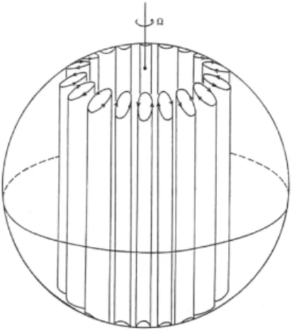
Fig. 1.2:A columnar structure alined with the rotation axis in a rotating sphere (Busse, 1970).

(27)

Fig. 1.3:The sketch of magnetogeostrophic flow viewed from the Northern hemisphere. Red and blue circles indicate clockwise anticyclone and counterclockwise cy-clone columns, respectively. Green, yellow, and white arrows show the Coriolis force, pressure gradient, and magnetic pressure, respectively. Magnetic field is concentrated inside anticyclone column because the Coriolis force faces in the direction of the center of the column.

(28)

Fig. 1.4:The geomagnetic field spectrum at the surface and the CMB in expansion of spherical harmonic degrees n. The curves represent the trend of observations at the Earth’s surface and extrapolations to the CMB (Langel and Estes, 1982).

(29)

Chapter 2 Method

2.1 Governing equations

In the present study, we use a numerical geodynamo model given by an electrically

conducting Boussinesq fluid in a rotating spherical shell. The governing equations

of the geodynamo in the outer core are described by the momentum equation, heat

equation, continuity equation, magnetic induction equation, and Gauss’s law for

the magnetic field, which are respectively given as

ρ0 ( ∂u ∂t + (u· ∇)u ) =−∇P + ρ0ν∇2u + ρg− 2ρ0Ω× u + J × B, (2.1) ∂T ∂t + (u· ∇)T = κT∇ 2_T, _(2.2) ∇ · u = 0, (2.3)

(30)

∂B

∂t =∇ × (u × B) + η∇

2_B, _(2.4)

and

∇ · B = 0, (2.5)

where u, B, J , g, T, P, ρ, αT, Ω, ν, κT, and η are velocity, magnetic field, current

density, acceleration of gravity, temperarure, pressure, mass density, thermal

ex-pansion rate, rotation angular velocity, kinematic viscosity, thermal diffusivity,

and magnetic diffusivity, respectively, and ρ0 is the stationary component of the

density. Since the Boussinesq approximation is applied in (2.1), the density

varia-tion due to temperature is only related to the buoyancy term. The mass density ρ is

written as a function of T as ρ = ρ0[1− αT(T− T0)], where T0is the temperature

of a reference state.

We normalize the length, time, temperature, pressure, and magnetic field by

the outer core thickness, L(= ro − ri), kinematic viscous diffusion time, L2/ν,

average temperature difference between the ICB and the CMB, ∆T , the pressure

by ν2/L2_{, and the magnetic field by}√_ρ

(31)

governing equations is given as ∂u ∂t + (∇ × u) × u = −∇ ( P + 1 2u 2 ) − ∇ × (∇ × u) +Ra P rT r ro − 2 Eez× u + 1 P m· E(∇ × B) × B, (2.6) ∂T ∂t =−(u · ∇)T + 1 P r∇ 2_T, _(2.7) ∇ · u = 0, (2.8) ∂B ∂t =∇ × (u × B) − 1 P m∇ × (∇ × B), (2.9) and ∇ · B = 0. (2.10)

The Rayleigh number, Ra, Ekman number, E, Prandtl number, P r, and magnetic

Prandtl number, P m are respectively defined as follows:

Ra = αTg0(∆T )L 3 νκT , E = ν ΩL2, P r = ν κT , P m = ν η. (2.11)

(32)

We use a numerical dynamo code Calypso (Matsui et al., 2014) for the

com-putation of the governing equations. The outer core is modeled in the

three-dimensional spherical coordinate (r, θ, ϕ). The spherical harmonic expansion is

used for the horizontal discretization. A scalar field, for example, temperature

T (r, θ, ϕ) is expanded as T (r, θ, ϕ) = lmax ∑ l=0 l ∑ m=−l T_lm(r)Y_lm(θ, ϕ). (2.12) The spherical harmonics Ym

l are defined as real functions. Plmcos(mθ) is

as-signed for positive m, P_lmsin(mθ) is assigned for negative m, where P_lmare the Schmidt quasi-normalized associated Legendre functions. Because of (2.8) and

(2.10), velocity and magnetic field are solenoidal fields, which can be decomposed

into poloidal and toroidal components. For example, magnetic field is expressed

by B(r, θ, ϕ) = lmax ∑ l=1 l ∑ m=−l (B_Slm+ B_{T l}m), (2.13) where B_Slm(r, θ, ϕ) =∇ × ∇ × (B_Slm(r)Y_lm(θ, ϕ)er), (2.14)

(33)

and

B_{T l}m(r, θ, ϕ) =∇ × (B_{T l}m(r)Y_lm(θ, ϕ)er). (2.15)

Now er is a unit vector in the radial direction. The orthogonality relations for the

spherical harmonics Ym

l , the poloidal field (e.g., BSlm), and the toroidal field (e.g.,

B_{T l}m) are ∫ ∫ Y_lmY_lm′ ′sin θdθdϕ = 4π 1 2l + 1δll′δmm′, (2.16) ∫ ∫ B_Slm· B_Slm′′sin θdθdϕ = Nl 1 r2 [ l(l + 1) r2 |B m Sl| 2₊∂BSlm ∂r 2]δll′δmm′, (2.17) ∫ ∫ B_{T l}m· B_{T l}m′′sin θdθdϕ = Nl 1 r2|B m T l| 2_δ ll′δmm′, (2.18) and ∫ ∫ B_Slm· B_{T l}m′′sin θdθdϕ = 0, (2.19)

where δll′ is Kronecker delta and Nl = 4πl(l + 1)/(2l + 1). The second-order

(34)

For the time integration, the Crank-Nicolson method is used in the linear diffusive

terms and the second order Adams-Bashforth method is used in the other terms.

2.2 Initial and boundary conditions

For the initial condition, temperature perturbation was applied to all sectorial

modes given by l = |m|. The initial magnetic field was set as an axial dipole plus a zonal toroidal field based on Christensen et al. (2001). For the boundary

condition, simulations were performed with fixed temperature (FT) boundary and

fixed heat flux (FF) boundary. In FT cases, the temperatures at the CMB were

fixed as T₀0(ro) = 1 and Tlm(ro) = 0 for l≥ 1. The temperatures at the ICB were

also fixed as T_lm(ri) = 0 for l ≥ 0. In FF cases, the radial temperature gradient

was set as ∂T0

0/∂r = A, and ∂Tlm/∂r = 0 for l ≥ 1, where A is a constant heat

flux. The mantle and inner core were assumed to be co-rotating, and a non-slip

boundary (u = 0) was applied to the CMB and ICB, i.e., the poloidal and toroidal

coefficients of velocity, Um

Sl(r) and USTm(r) were set as USlm(r) = ∂USlm/∂r = 0

and U_{T l}m(r) = 0 at the CMB and ICB. The mantle and inner core were assumed to be electrically insulated, and the magnetic field at the boundaries was connected

to the potential field, i.e., the poloidal and toroidal coefficients of magnetic field,

Bm

(35)

parameter setting, Ra was changed among the cases; the Ekman, Prandtl, and

magnetic Prandtl numbers were fixed at E = 1× 10−3, P r = 1, and P m = 5 in all simulation cases. The truncation of the spherical harmonics and the radial grid

points were set to lmax = 47 and Nr = 63, respectively. To avoid aliasing in the

spherical harmonic expansion, horizontal grids were set to (Nθ, Nϕ) = (72, 144).

To investigate the effects of different inner core sizes, the spherical shell radius

ratios of the inner core radius to the outer core radius were set as ri/ro = 0.15,

0.25, and 0.35. The inner and outer core radii, riand ro, were defined by

ri= ri/ro 1− ri/ro , ro = 1 1− ri/ro . (2.20)

In each radius ratio case, ri and ro were set as Table 2.1. First, we performed

numerical simulations of non-magnetic thermal convection in rotating spherical

shells to estimate the critical Rayleigh number, Racrit, for the onset of thermal

convection. We then carried out numerical simuations of magnetohydrodynamic

(MHD) dynamos driven by the thermal convection.

Table 2.1:Spherical shell dimensions for various values of ri/ro.

ri/ro ri ro L

0.15 3/17(= 0.1764705882352941) 20/17(= 1.1764705882352941) 1 0.25 1/3(= 0.3333333333333333) 4/3(= 1.3333333333333333) 1 0.35 7/13(= 0.5384615384615384) 20/13(= 1.5384615384615384) 1

(36)

Chapter 3 Fixed temperature

3.1 Result of thermal convection

First, we performed numerical simulations of non-magnetic thermal convection

in order to estimate the critical Rayleigh number (Racrit), the Rayleigh number

required for the onset of the thermal convection. We solved the set of equations of

(2.6) without the Lorentz force term, (2.7), and (2.8). The kinetic energy density

was calculated by Ekin = 1 2VS ∫ VS u2dV, (3.1)

where VS is the volume of the spherical shell, for the average in the time interval

from t/τν = 4.5 to 6, where τν is the viscous diffusion time.

(37)

numbers are estimated to be Racrit = 1.09× 105, 0.72× 105, and 0.56× 105 in

ri/ro = 0.15, 0.25, and 0.35, respectively, by the method used in Al-Shamali et al.

(2004). The obtained values of Racritare almost identical to those reported in

Al-Shamali et al. (2004) for the same parameters and conditions used in this study.

We obtain larger Racrit for the smaller aspect ratio, indicating that the convection

in a rotating, thick spherical shell requires large buoyancy. Ekinlisted in Table3.2

are results of larger Ra cases than those in Table3.1.

3.2 Result of MHD simulation

We performed MHD dynamo simulations for various Rayleigh numbers and the

radius ratios using Eqs. (2.6)-(2.10). The magnetic energy density was calculated

by Emag = 1 2VSEP m ∫ VS B2dV. (3.2)

Tables 3.3, 3.4, and 3.5 list results of MHD simulations. First, we changed the

amplitude of the initial magnetic field, Binit = 0.3, 0.5, 0.7, and 1, at Racrit = 2.5

for ri/ro = 0.25. The time evolution of the kinetic and magnetic energy densities

in each Binit is shown in Fig. 3.2. When large Binit were set, Ekin and Emag

(38)

we adopted Binit = 1. We performed numerical simulations for the time interval

at least two magnetic diffusion times (t = 2τη = 2P mτν) to assess whether the

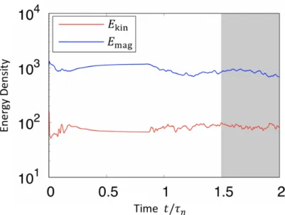
magnetic field was sustained or dissipated. Fig.3.3 shows the time evolution of

the kinetic and magnetic energy densities at Racrit = 2.8 for ri/ro = 0.25, as an

example of the case where the magnetic field was sustained. We calculated the

time average of the kinetic and magnetic energy densities as well as the dipolarity

over the 0.5 magnetic diffusion time at the end of simulations, the time interval

indicated by the shaded area in Fig.3.3. The kinetic and magnetic energy densities

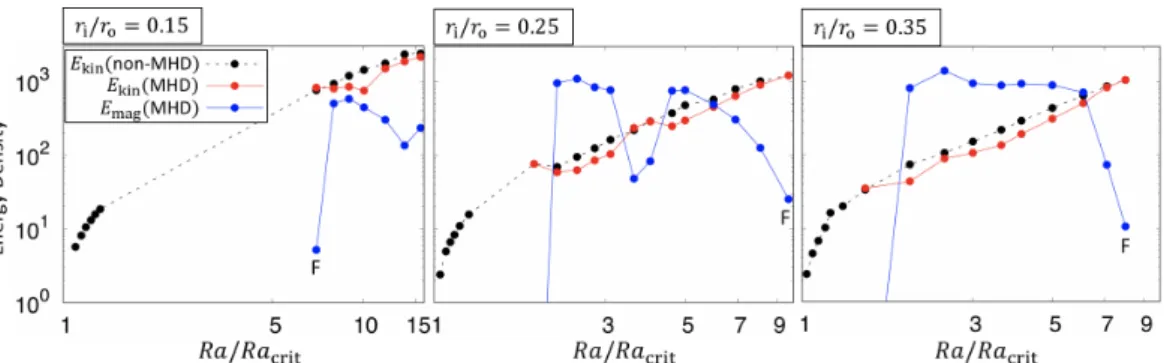
as a function of the Rayleigh number are shown in Fig. 3.4, where the black,

red, and blue points are the Ekin in the non-MHD cases, Ekin in the MHD cases,

and Emag in the MHD cases, respectively. The ”F” denotes the failed dynamo

cases. In each radius ratio case with a sustained magnetic field, the Ekinvalues in

the MHD cases are smaller than the Ekin values in the corresponding non-MHD

cases. These results show that the Lorentz force caused by the intense magnetic

field disturbs convection. We also find the different tendency of the kinetic and

magnetic energy densities among the three radius ratio cases. At ri/ro = 0.15,

the Emag values in the MHD cases are smaller than the Ekin values in the MHD

cases for all cases. This trend is consistent with the results of Heimpel et al.

(39)

significantly smaller than those for the cases of other Rayleigh numbers. Although

the trend in the magnetic energy spectrum does not change, there is a decrease in

the amplitude. At ri/ro = 0.35, the values of Emag in the MHD cases are larger

than the values of Ekin in the MHD cases for almost all cases. The results of the

different ri/ro indicate that it is not likely to sustain a strong magnetic field with

a smaller inner core.

To examine dynamics of the outer core, we calculated the Elsasser number Λ,

which is the ratio of the Lorentz force to the Coriolis force. The Elsasser number

is acquired by

Λ = B

2

ρ0µ0ηΩ

= 2P mEEmag. (3.3)

Fig. 3.5 shows Λ as a function of the Rayleigh number for different spherical

shell geometries. The red, blue, and green points indicate the cases of ri/ro =

0.15, 0.25, and 0.35, respectively. The range of Λ is approximately from 5 to 10

in sustained strong dipole dynamo cases in all ratios, indicating that the Lorentz

force is sufficiently working for core dynamics. At ri/ro = 0.15, even though the

magnetic energy is smaller than kinetic energy, Λ is larger than one and therefore

the Lorentz force is significantly working as well.

To examine the dynamo occurring condition, we calculated the magnetic Reynolds

(40)

induction equation. The magnetic Reynolds number is acquired by

Rm = U L

η =

√

2EkinP m. (3.4)

Fig. 3.6 shows Rm as a function of the Rayleigh number for different spherical

shell geometries. The red, blue, and green circles indicate Rm values in the cases

of ri/ro = 0.15, 0.25, and 0.35, respectively. We found that Rm increases with

increasing the Rayleigh number in all radius ratio cases. The range of Rm for

sustained dynamos was Rm > 193.4 at ri/ro = 0.15, Rm > 54.3 at ri/ro =

0.25, and Rm > 46.7 at ri/ro = 0.35. This is consistent with the numerical

simulation results of Olson et al. (2006) that the minimum Rm is approximately

39 at ri/ro = 0.35. The minimum Rm for sustained dynamos becomes larger

with the smaller inner core, indicating that larger generation term in the induction

equation is needed to defeat magnetic diffusion with the smaller inner core.

Magnetic moment M is calculated from Eq. (1.3). From the Preliminary

Ref-erence Earth Model (Dziewonski and Anderson, 1981), the density in the outer

core is 10 − 12 g/cm3₍≈ 104 _kg/m3_{), so we use ρ}

0 = 104 kg/m3. The

mag-netic permeability in vacuum is a constant; µ0 = 4π× 10−7 H/m. The

rota-tion angular velocity Ω = 2π/1 day = 7.27 × 10−5/s. The magnetic

(41)

5 are acquired from this magnetic field scaling.

To verify whether the truncation of lmax = 47 is sufficient resolution, we

performed simulations for Ra/Racrit = 2.0 at ri/ro = 0.35 with lmax = 47 and

95. Spectra of kinetic and magnetic energy densities are shown in Figs.3.7 and

3.8. The spectrum with lmax = 47 is almost the same as that with lmax = 95 for

l ≤ 47. This truncation is found to be enough to solve dynamo simulations in this

control parameter setting.

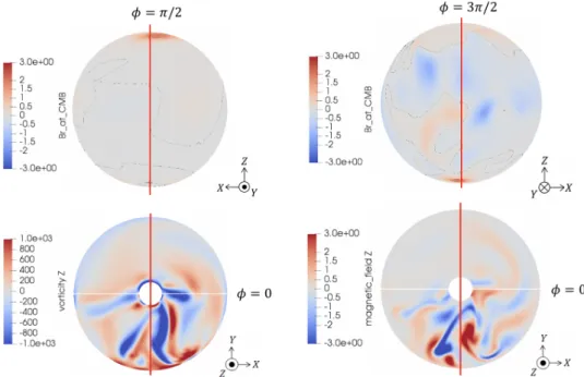
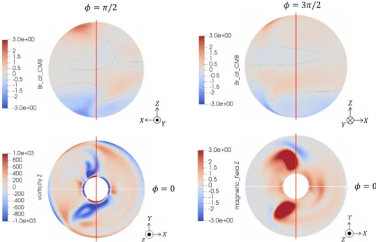
Fig.3.9shows the radial component of the magnetic field at the CMB and the

equatorial cross-sections of the z-component of the vorticity and magnetic field

are plotted at Ra/Racrit = 11.9 for ri/ro = 0.15. The same plots at Ra/Racrit=

3.1 for ri/ro = 0.25 and at Ra/Racrit = 3.0 for ri/ro = 0.35 are shown in

Figs 3.10and3.11, respectively. Spectra of kinetic and magnetic energy density

are shown in Figs 3.12, 3.13, and 3.14. At the equatorial plane, the magnetic

field is concentrated in the anti-cyclone columns to generate a dipolar field at

ri/ro = 0.25 and 0.35; intense magnetic patches are located near the tangent

cylinder, which is an imaginary cylinder tangent to the inner-core equator and

coaxial with the rotation axis. In the case of ri/ro = 0.15, strong convection is

generated locally, where strong BZ convection is generated between the cyclonic

and anti-cyclonic columns in the equatorial plane. As these intense magnetic fields

are not concentrated in the convection columns, the radial magnetic field at the

(42)

equator) and is smaller than that of the cases with different aspect ratios.

3.3 Assessment of dipolar dominance

In numerical dynamos, dipolarity is used for quantification of the magnetic field

morphology at the CMB. Although the dipolarity has been evaluated in some

nu-merical dynamos (Christensen and Aubert, 2006; Soderlund et al., 2012), it is

not sufficiently valid in dynamos whose dipolarities are gradually changing (e.g.,

Aubert et al., 2009). In an observational study of the geomagnetic field, the dipole

is assessed by how far the dipolar component is from the trend of higher degree

components (Lowes 1974; Langel and Estes, 1982). We quantitatively evaluated

the dipolar component dominance in combination with the dipolarity, comparison

of the dipolar magnetic energy, and an extrapolation of l = 1 based on the fitting

curve for higher degrees. To quantitatively evaluate the axial dipole component

dominancy, we calculated the dipolarity at the CMB, defined by

fdip= ( Emag(l=1,m=0)(r = ro) ∑lmax l=1 ∑l m=0E (l,m) mag (r = ro) )1/2 , (3.5)

where Emag(l,m)(r = ro) is the magnetic energy of (l, m) component at the CMB.

(43)

CMB, Emag(r = ro), is calculated by Emag(r = ro) = 1 2SoEP m ∫ S B2dS, (3.6)

where So(= 4πro2) is the area of the CMB. Fig.3.15 shows the dipolarity as a

function of the Rayleigh number for ri/ro = 0.15, 0.25, and 0.35. The dipolarity

gradually decreases with increasing Rayleigh number for ri/ro = 0.25 and 0.35.

The axial dipolar component becomes weak during intense convection. The

de-pendency of the dipolarity on the Rayleigh number is similar for the radius ratio

cases of ri/ro = 0.25 and 0.35. Here, fdipis always larger than 0.35 in the cases of

ri/ro = 0.25 and 0.35. In contrast, we find the different tendency in ri/ro = 0.15;

fdipis larger than 0.45 at Ra/Racrit = 8.0 and 9.0 while fdipis smaller than 0.35

at Ra/Racrit > 10.1.

Previous numerical dynamo simulations used the threshold of the dipolar

dom-inance for fdip = 0.35. To obtain a clearer threshold for the dipole dominancy,

we focused on the magnetic energy spectrum at the CMB as a function of the

spherical harmonic degree, l. For example, Fig.3.16 shows the magnetic energy

density as a function of the spherical harmonic degree at Ra/Racrit = 2.8 for

ri/ro = 0.25. Using odd-degree components in the magnetic energy from l = 3

to 19, we evaluated a fitting curve as 46.21 × 1.481−l. We compared the Emag

of the simulation result at l = 1 (El=1

(44)

function (E_{mag fitting}l=1 ). Then, we acquired the ratio of Emag for the simulation

re-sult to that from the extrapolated value, E_{mag data}l=1 /E_{mag fitting}l=1 (hereafter referred to as fmag fit). We can assess the dipolar component dominance from a higher

de-gree trend based on how much the ratio of the extrapolation from fitting fmag fitis

larger than 1. Here, fmag fitwas calculated in all cases and plotted as a function of

the Rayleigh number at ri/ro = 0.15, 0.25, and 0.35 (Fig.3.17). At ri/ro = 0.15,

fmag fit was smaller than 1 at Ra/Racrit > 10.1. At ri/ro = 0.25, fmag fit was

approximately 2.1 at Ra/Racrit = 2.2 and gradually decreased to 1.6 with

in-crease of Ra/Racrit of up to approximately 8.0. At ri/ro = 0.35, fmag fit was

approximately 4.7 at Ra/Racrit = 2.0, gradually decreasing to 2.1 with increase

of Ra/Racritup to approximately 7.0.

Comparing the result between fdipand fmag fit, we find that the dipolar

domi-nane decreases with increasing Rayleigh number. At ri/ro = 0.15, weak dipolar

dominancy can be represented by Ra/Racrit > 10.1 for both indices. We note

the different behavior of fdip and fmag fit in the smaller Ra/Racrit range in the

different ri/rocases; the fdipvalues obtained in ri/ro = 0.25 are larger than those

in ri/ro = 0.35, while the fmag fit values obtained in ri/ro = 0.25 are smaller

than those in ri/ro = 0.35. The different behavior of fdipand fmag fitcan be

(45)

ri/ro = 0.25 and 0.35, Emag datal=1 is significantly large at ri/ro = 0.35, and

there-fore fmag fitis large at ri/ro = 0.35 than at ri/ro = 0.25. The difference between

fdipand fmag fit is whether a higher-degree spectrum is taken into account or not.

The dependence of the dipolar dominance on the radius ratio can be revealed by

fmag fitas it contains information obtained from a higher degree spectrum.

We show an example in which we could not categorize the dipole or

non-dipole based only on the dipolarity, i.e., the cases for fdip = 0.376 at Ra/Racrit=

7.1 with ri/ro = 0.35 and fdip = 0.349 at Ra/Racrit = 10.1 for ri/ro = 0.15.

Fig. 3.18shows the CMB spectra for these two cases. The dipolar component is

dominant against the high degree trend in the former case while it is not dominant

in the latter case. The ratio of extrapolation from the fitting is fmag fit = 2.071

in the former case and fmag fit = 0.860 in the latter case; we observed that the

former case is dipolar-dominated while the latter case is non-dipolar dominated.

The results of fmag fitalso indicate the dependence of the dipolar dominance on the

inner core size. The dipolar dominance becomes weaker with a smaller inner core

by calculating the dipolar magnetic energy at the CMB (Heimpel et al., 2005). On

the other hand, this tendency is not obvious in the results of fdip.

Consideration using both fdipand fmag fitenables us to categorize the dynamo

regime of the simulation results quantitatively. The results of the categorization

of the dynamo regime are shown in Fig. 3.19, where the red circles, blue

(46)

non-dipolar, and failed dynamo cases, respectively. We categorized strong

dipo-lar when the magnetic energy is dipo-larger than the kinetic energy in each simulation

result, and vice versa. Sustaining the dynamo with a smaller inner core size

re-quires a larger Rayleigh number. This is consistent with the findings of Heimpel

et al. (2005). At ri/ro = 0.35, almost all the sustained dynamo cases were strong

dipoles. At ri/ro = 0.25, there were strong dipolar dynamo cases and weak

dipo-lar dynamo cases. At ri/ro = 0.15, there were weak dipolar and non-dipolar

dynamo cases.

3.4 Discussion

The dipolarity at the CMB of the present Earth is fdip= 0.64, which is calculated

from the 13th IGRF model (Alken et al., 2021). The present radius ratio, ri/ro, is

0.35. The range of the dipolarity calculated from results of our numerical

simu-lations of geodynamo for ri/ro = 0.25 and 0.35 covers the present Earth’s

dipo-larity. The morphology of the sustained magnetic field in both ratios is Earth-like.

The ratio of the extrapolation from fitting in the present Earth is fmag fit = 4.925.

Here, fmag fit is larger than approximately half of the present Earth’s value for

almost all the cases at ri/ro = 0.35 while fmag fit is smaller than that of almost

(47)

ri/ro = 0.25 than the present Earth. In contrast, the dipolarity at ri/ro = 0.15 is

smaller than the present Earth’s dipolarity in all cases. The dipole component is

not dominant.

In numerical dynamos at ri/ro = 0.35, we verified that the transition between

the dipole and non-dipole is fdip ≈ 0.35 (Christensen and Aubert, 2006; Olson et

al., 2011). Our results are consistent with this transition. While dipolarity is an

ef-fective index if dynamos can be categorized into large and small dipolarity groups,

the combination of dipolarity and the ratio of extrapolation from fitting assesses

the dipolar dominance if the dipolarity changes gradually, as in our results.

At ri/ro = 0.15, an axial dipole field formed by a single column (Heimpel

et al., 2005). In this study, a dipole field is also formed by some azimuthally

localized narrow columns around the dynamo-onset cases. Emag is found to be

always smaller than Ekinin all Ra cases. The magnitude relationship is the same

as that of Heimpel et al. (2005). A strong dipole is sustained with a smaller inner

core in the fixed flux calculation (Hori et al., 2010), changing the core power based

on the thermal history (Driscoll, 2016), or the buoyancy gained by light elements

(Lhuillier et al., 2019). Clarifying how heat flow at boundaries sustains the dipole

requires further numerical simulations.

Our proposed method of evaluating the dipolar dominance, fmag fit, enables

quantitative investigations of the magnetic field structure in the past environment.

(48)

ge-omagnetic pole), is acquired based on the assumption that the gege-omagnetic field

was dipolar-dominated in the past (Merrill et al., 1996). In contrast, the VGP paths

and actual behavior of the geomagnetic field are not dipolar-dominant.

Investiga-tion of the numerical dynamo with our proposed method is capable of improving

the understanding of the actual behavior of the geomagnetic field and

(49)

Table 3.1:Results of Ekin for thermal convection at t = 6τν in ri/ro= 0.15, 0.25, and

0.35 under the FT boundary condition. ri/ro Ra[×105] Ekin 0.15 1.0 8.31× 10−6 0.15 1.2 5.72 0.15 1.25 8.15 0.15 1.3 10.62 0.15 1.35 13.16 0.15 1.4 15.80 0.15 1.45 18.54 0.25 0.70 8.55× 10−4 0.25 0.75 2.41 0.25 0.78 4.94 0.25 0.80 6.62 0.25 0.82 8.35 0.25 0.85 11.02 0.25 0.90 15.70 0.35 0.55 1.76× 10−4 0.35 0.58 2.38 0.35 0.60 4.54 0.35 0.62 6.76 0.35 0.65 10.22 0.35 0.67 12.60 0.35 0.70 16.28

(50)

Table 3.2:Results of Ekinin ri/ro= 0.15, 0.25, and 0.35.

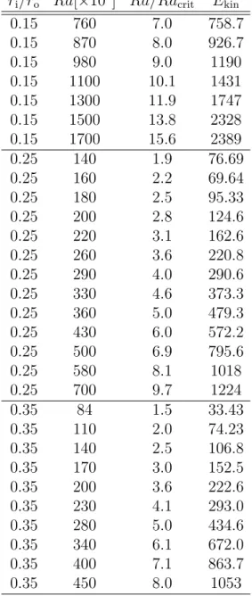
ri/ro Ra[×105] Ra/Racrit Ekin

0.15 760 7.0 758.7 0.15 870 8.0 926.7 0.15 980 9.0 1190 0.15 1100 10.1 1431 0.15 1300 11.9 1747 0.15 1500 13.8 2328 0.15 1700 15.6 2389 0.25 140 1.9 76.69 0.25 160 2.2 69.64 0.25 180 2.5 95.33 0.25 200 2.8 124.6 0.25 220 3.1 162.6 0.25 260 3.6 220.8 0.25 290 4.0 290.6 0.25 330 4.6 373.3 0.25 360 5.0 479.3 0.25 430 6.0 572.2 0.25 500 6.9 795.6 0.25 580 8.1 1018 0.25 700 9.7 1224 0.35 84 1.5 33.43 0.35 110 2.0 74.23 0.35 140 2.5 106.8 0.35 170 3.0 152.5 0.35 200 3.6 222.6 0.35 230 4.1 293.0 0.35 280 5.0 434.6 0.35 340 6.1 672.0 0.35 400 7.1 863.7 0.35 450 8.0 1053

(51)

T able 3.3: Results of Ekin ,E mag , and fdip for MHD dynamos at ri /r o = 0 .15 under the FT boundary condition. ri /r o R a [× 10 3 ] R a/R acrit Ekin Emag Λ R m fdip fmag fit M [ZAm 2 ] 0 .15 440 4 .0 297 .1 3 .244 0 .0324 121 .9 − − − 0 .15 760 7 .0 823 .7 5 .193 0 .0519 202 .9 − − − 0 .15 870 8 .0 801 .4 501 .6 5 .02 200 .2 0 .494 1 .435 70 .06 0 .15 980 9 .0 846 .4 579 .0 5 .79 205 .7 0 .516 1 .866 75 .20 0 .15 1100 10 .1 748 .4 444 .7 4 .45 193 .4 0 .349 0 .860 27 .69 0 .15 1300 11 .9 1493 300 .5 3 .01 273 .2 0 .117 0 .322 13 .04 0 .15 1500 13 .8 1867 135 .6 1 .36 305 .5 0 .155 0 .391 9 .155 0 .15 1700 15 .6 2141 234 .3 2 .34 327 .2 0 .172 0 .420 14 .67

(52)

T able 3.4: Results of Ekin ,E mag , and fdip for MHD dynamos at ri /r o = 0 .25 under the FT boundary condition. ri /r o R a [× 10 3 ] R a/R acrit Ekin Emag Λ R m fdip fmag fit M [ZAm 2 ] 0 .25 140 1 .9 76 .69 1 .491 × 10 − 4 1 .491 × 10 − 6 61 .68 − − − 0 .25 160 2 .2 59 .05 958 .6 9 .59 54 .33 0 .860 2 .116 270 .4 0 .25 180 2 .5 62 .89 1097 10 .97 56 .08 0 .867 2 .397 286 .4 0 .25 200 2 .8 85 .49 844 .4 8 .44 65 .38 0 .784 1 .828 221 .9 0 .25 220 3 .1 103 .9 769 .2 7 .69 72 .08 0 .757 2 .441 200 .0 0 .25 260 3 .6 236 .4 48 .4 0 .484 108 .7 0 .644 2 .477 34 .87 0 .25 290 4 .0 289 .3 83 .0 0 .830 120 .3 0 .620 2 .610 41 .30 0 .25 330 4 .6 248 .6 753 .8 7 .54 111 .5 0 .602 2 .287 103 .3 0 .25 360 5 .0 297 .7 769 .0 7 .69 122 .0 0 .562 1 .935 146 .6 0 .25 430 6 .0 455 .6 491 .0 4 .91 150 .9 0 .522 1 .887 83 .72 0 .25 500 6 .9 642 .2 305 .2 3 .05 179 .2 0 .456 1 .551 62 .10 0 .25 580 8 .1 906 .8 126 .0 1 .26 212 .9 0 .412 1 .556 50 .84 0 .25 700 9 .7 1221 25 .4 0 .254 247 .1 − − −

(53)

T able 3.5: Results of Ekin ,E mag , and fdip for MHD dynamos at ri /r o = 0 .35 under the FT boundary condition. ri /r o R a [× 10 3 ] R a/R acrit Ekin Emag Λ R m fdip fmag fit M [ZAm 2 ] 0 .35 84 1 .5 35 .09 2 .376 × 10 − 3 2 .376 × 10 − 5 41 .89 − − − 0 .35 110 2 .0 43 .61 819 .6 8 .20 46 .70 0 .816 4 .713 297 .6 0 .35 140 2 .5 89 .35 1408 14 .1 66 .83 0 .724 3 .174 356 .0 0 .35 170 3 .0 106 .8 950 .2 9 .50 73 .08 0 .739 4 .239 236 .8 0 .35 200 3 .6 136 .3 890 .2 8 .90 82 .55 0 .692 3 .900 200 .3 0 .35 230 4 .1 193 .1 938 .4 9 .38 98 .26 0 .632 2 .946 203 .4 0 .35 280 5 .0 311 .9 895 .6 8 .96 124 .9 0 .556 2 .848 162 .3 0 .35 340 6 .1 508 .7 713 .6 7 .14 159 .5 0 .480 2 .006 132 .7 0 .35 400 7 .1 837 .6 73 .46 0 .735 204 .7 0 .376 2 .071 24 .92 0 .35 450 8 .0 1060 10 .61 0 .106 230 .2 − − −

(54)

Fig. 3.1:The kinetic energy density, as a function of the Rayleigh number, calculated in spherical shells with different geometries. Red, green, and blue lines indicate the linear fitting for ri/ro = 0.15, 0.25, and 0.35, respectively.

(55)

Fig. 3.2:Time evolution of energy density in various amplitudes of the initial magnetic field at Ra/Racrit= 2.5 at ri/ro = 0.25.

Fig. 3.3:Time evolution of energy density in the case of sustained dynamo at Ra/Racrit = 2.8 at ri/ro = 0.25. The red and blue lines denote the kinetic

(56)

Fig. 3.4:The kinetic and magnetic energy density as a function of the Rayleigh number in spherical shells with different geometries. The black, red, and blue points are the Ekin values in the non-MHD cases, Ekin values in the MHD cases, and

Emagvalues in the MHD cases, respectively. The ”F” denotes the failed dynamo

cases.

Fig. 3.5:The Elsasser number Λ as a function of the Rayleigh number for different spher-ical shell geometries. The red, blue, and green circles indicate Lambda values for the cases of ri/ro= 0.15, 0.25, and 0.35, respectively.

(57)

Fig. 3.6:The magnetic Reynolds number Rm as a function of the Rayleigh number for different spherical shell geometries. The red, blue, and green circles indicate Rm values for the cases of ri/ro = 0.15, 0.25, and 0.35, respectively.

(58)

Fig. 3.7:Spectrum of the kinetic and magnetic energy density for the case with Ra/Racrit = 2.0 at ri/ro = 0.35 and lmax = 47. The red and blue lines

denote the kinetic and magnetic energy density, respectively.

Fig. 3.8:Spectrum of the kinetic and magnetic energy density for the case with Ra/Racrit = 2.0 at ri/ro = 0.35 and lmax = 95. The red and blue lines

(59)

Fig. 3.9:Spatial pattern of the flow and magnetic fields for the case with Ra/Racrit =

11.9 at ri/ro = 0.15. The radial magnetic field, Br, at the CMB, viewed from

ϕ = π/2 and 3π/2, are plotted in the upper left and right, respectively. The z component of the vorticity, ωZ, and magnetic field, BZ, at the equatorial plane

(60)

(61)

(62)

Fig. 3.12:Spectrum of the kinetic and magnetic energy density at t/τη = 2.0 for the case

with Ra/Racrit = 11.9 at ri/ro = 0.15. The red and blue lines denote the

kinetic and magnetic energy density, respectively.

(63)

東北大学機関リポジトリTOUR

Dominance of a dipole magnetic field under the

condition of the past Earth's interior based

on numerical simulations of the geodynamo

著者

Nishida Yuki

学位授与機関

Tohoku University

博士論文

Dominance of a dipole magnetic field under

the condition of the past Earth’s interior based

on numerical simulations of the geodynamo

（数値ダイナモシミュレーションに基づく

過去の地球内部条件下における

双極子磁場卓越性に関する研究）

博士論文

Dominance of a dipole magnetic field under

the condition of the past Earth’s interior based

on numerical simulations of the geodynamo

（数値ダイナモシミュレーションに基づく

過去の地球内部条件下における

双極子磁場卓越性に関する研究）

東北大学大学院理学研究科

地球物理学専攻

西田 有輝

令和

2

年

Acknowledgement

Abstract

Contents

Chapter 1

Introduction

1.1

Development of dynamo studies

1.2

Observations of a magnetic field

1.3

Properties of the outer core

1.4

Focusing on the inner core size

1.5

Purpose of this study

Name

Definition

Ratio

Estimation

Rayleigh

number

R

a

=

α

g

(∆

T

)L

/ν

κ

b

uo

yanc

y

vs

viscous

forces

10

Ekman

number

E

=

ν

/

Ω

L

viscous

vs

Coriolis

forces

10

西田有輝