THE MODULI SPACE OF ONCE PUNCTURED ELLIPTIC CURVES WITH LAGRANGIAN SUBLATTICES

THE MODULI SPACE OF ONCE PUNCTURED ELLIPTIC CURVES

WITH LAGRANGIAN SUBLATTICES

YOSHITAKE HASHIMOTO (橋本義武) AND KIYOSHI OHBA (大場清)

1. INTRODUCTION

We introduced a new method ofconstructing once punctured Riemann surfaces in

[H-Ol] (see also [H-O2]). In our construction we use line segments in the complex plane

$\mathbb{C}$ and parallel transformations: For a pair of disjoint parallel line segments with the

same length in $\mathbb{C}$, we first cut $\mathbb{C}$ along the segments and paste each side ofone segment

and the opposite side of the other segment by a parallel transformation obtaining a once

punctured elliptic curve. The puncture is at infinity. We shall call such a pair an Igeta.

(Igetais aJapanesewordcomingfrom atechnical term “Igeta-kuzushi” used in aJapanese

martial art.) Putting$g$disjoint pieces ofIgeta on $\mathbb{C}$, we obtainaonce punctured Riemann

surface of

genus

$g$ in the salne way. (See Figure 1. The numbers (1),$\ldots,(6)$ in Figure 1

indicate where to paste.) We denote a set of$g$ disjoint Igeta by $\Gamma$ and the resulting once

punctured Riemann surface by $(R(\Gamma),p_{\infty})$. Moreover when we

move

the position of $g$

Igeta, there appears a family of once punctured Riemann surfaces of

genus

$g$. All the

possible configurations of $g$ disjoint Igeta up to the affine automorphisms of $\mathbb{C}$ form a

$3g-2$-dimensional complex $\iota\nearrow$-manifold and this dimension is the same as the dimension

of the moduli space $\mathcal{M}_{g,1}$ ofoncepunctured Rielnann surfaces ofgenus $g$

.

We thusexpect

to have avisual image ofthe lnoduli space by using this construction.

Let $I_{g}\eta_{0}$ be the collection of those $\Gamma$ having $[0,1]$ as one of its _$2g$ line segments.

$I_{g}\eta_{0}$ turns out to be a $3g-2$-dimensional complex manifold. We showed in [H-O1] that the

Kodaira-Spencer map

$\rho_{\Gamma,0}$

:

$T(I_{g}\mathit{7}|_{0})_{\mathrm{r}}arrow H^{1}(R(\Gamma);(-p\infty))$

is an isomorphism for any $\Gamma\in I_{g}\eta_{0}$, where $T(I_{g}\eta_{0})_{\Gamma}$ is the holomorphic tangent space of

$I_{g}\eta_{0}$ at $\Gamma$ and _{$(-p_{\infty})$} is the sheaf ofgerms ofholomorphic vector fields on _$R(\Gamma)$ having

zero

at $p_{\infty}$. This implies that the family of

once

punctured Riemann surfaces of

genus

$g$

by Igeta-construction is $\mathrm{c}\mathrm{o}\mathrm{n}\mathrm{u}\mathrm{l}$)

$\mathrm{l}\mathrm{e}\mathrm{t}\mathrm{e}$ and effectively

parametrized at any point for each $g$.

We also showed that any once punctured Riemann surface $(R,p)$ can be obtained from

$\mathbb{C}$ by cutting along line segments and pasting by parallel transformations. (Note that

Igeta-construction is a special way of cutting and pasting.) This result is obtained by

considering a Lagrangian sublattice A of $R$, a subgroup of $H_{1}(R;\mathbb{Z})$ which coincides its

orthogonal $\mathrm{C}\mathrm{O}\ln_{\mathrm{P}^{1\mathrm{e}\mathrm{n}}}\mathrm{e}\mathrm{m}\mathrm{t}$with $1^{\cdot}\mathrm{e}\mathrm{s}_{\mathrm{P}^{\mathrm{e}\mathrm{c}\mathrm{t}}}$ to the intersection form

on

$H_{1}(R;\mathbb{Z})$.

When we construct a once punctured Riemann surface $(R(\Gamma),p_{\infty})$ from $\Gamma,$ $R(\Gamma)$ has

a natural Lagrangian sublattice $\Lambda_{\Gamma}$. Igeta-construction leads us to consider the moduli

space of once punctured Riemann surfaces with Lagrangian sublattices.

In this paper we consider the case of genus 1, and describe the moduli space using a

natural extension ofIgeta-construction, that is, we make a complete list of

once

puctured

$/$

$/$

$arrow$ cut $\nearrow\nearrow$ $\approx$ $(4)\backslash (3)$ (5) (6) $(3)\backslash ^{(4)}$ (6) (5) FIGURE 1. Igeta-construction

Theorem 1. Foranyoncepunctured ellipticcurve with a Lagrangian sublattice$(E,p, \Lambda)$,

there exists one and $onl\tau/one(E(a, b, x),p_{\infty’ 0}\Lambda)$ isomorphic to $(E,p, \Lambda)$.

For any once $\mathrm{p}\mathrm{u}\mathrm{n}\mathrm{c}\mathrm{t}_{\mathrm{U}\mathrm{l}\mathrm{e}}\mathrm{d}$ Riemann surface $(R,p)$, a Lagrangian sublattice A and the

puncture $p$ deternline a certain Abelian differential $\omega_{\Lambda}$ of the second kind up to scalars.

To prove Theorem 1 westudy the geolnetry ofgeodesics on once punctured elliptic curves

having metrics with conical singularities induced by the Abelian differentials $\omega_{\Lambda}$. For

each $(.E(a, b, x),p_{\infty}, \Lambda 0)$, all the closed geodesics can be described visually by using our

construction.

In

_{\S 3}

we consider the conuplex structure ofthe moduli space of

once

punctured elliptic

curves

with Lagrangian sublattices by using the description given in

\S 2.

The authors would lilie to thank the many people who have contributed ideas and

suggestionsfor this $\mathrm{m}\mathrm{a}\mathrm{n}\mathrm{u}\mathrm{s}\mathrm{C}\Gamma \mathrm{i}1^{)}\mathrm{t},$ anlongthem C. F. B\"odigheimer, V. Chueshev, K. Fukaya,

M. Furuta, A. Hattori, S.

Morita

and K. Ono. The authors would like to express their

gratitude to H. Helling for useful suggestions on how to improve the early drafts.

2. ELLIPTIC CURVES WITH LAGRANGIAN SUBLATTICES

In this section, we give a description of all the once punctured elliptic

curves

with

Lagrangian sublattices $.\mathrm{b}\mathrm{y}$ using a natural extension ofIgeta-construction.

We prepare some notations and ternls about the metrics induced by Abelian

$\gamma$ : [$0,11arrow R$ -line-segment ifits image contains

no

poles of and the integral $\int_{\gamma(0}^{\gamma(1)})\omega$

$\mathrm{d}\mathrm{e}\mathrm{p}\mathrm{e}\mathrm{n}\mathrm{d}_{\mathrm{S}}$

on

$t\in[0,1]\mathrm{l}\mathrm{i}\overline{\mathrm{n}}$early. We also call its image $\omega$-line-segment. Let us denote

by $g_{\omega}$ the flat metric on $R-\omega^{-1}(\infty)$ induced by the 2-form

$\frac{i}{2}\omega\wedge\overline{\omega}$, which has conical

singularities at $\omega^{-1}(0)$

.

Then $\omega$-line-segments are geodesics for $g_{\omega}$. Let us call a $\omega$

-line-segment $\gamma$ : $[0,1]arrow R-\omega^{-1}(\infty)\omega$-edgeif$\gamma([0,1])\cap\omega^{-1}(0)=\{\gamma(0), \gamma(1)\}$

.

Then closed

geodesics with respect to $g_{\omega}$ which contain some zeros of

$\omega$ consist of $\omega$-edges because

the integral of $\omega$ gives rise to a local isometry between $R-(\omega^{-1}(\infty)\cup\omega^{-1}(0))$ and

$\mathbb{C}$

.

An Abelian differential $\omega$ of the second kind

on

a closed Riemann surface $R$ induces

an element of $H^{1}(R;\mathbb{C})$, and further an elenuent denoted by $\mathrm{P}\mathrm{D}[\omega]$ of $H_{1}(R;\mathbb{C})$ via the

Poincar\’e duality. It holds that

$\int_{\alpha}\omega=\alpha\cdot \mathrm{P}\mathrm{D}[\omega]$ for any $\alpha\in H_{1}(R;\mathbb{Z})$

.

We look for a singular 1-cycle $\sigma$ representing $\mathrm{P}\mathrm{D}[\omega]$ such that

$\sigma=\sum_{k=1}^{N}ck.\gamma_{k}.$, $c_{k}\in \mathbb{C}$

where $\gamma_{1},$ $\ldots,\gamma_{N}$ are $\omega$-edges. (We can find it if$\omega^{-1}(0)$ is nonempty.)

Let $(R,p)$ be

a once

punctured Rielnann surface of

genus

$g$ and A

a

Lagrangian

sub-lattice of $H_{1}(R;\mathbb{Z})$. The kernel $Z_{\Lambda}$ ofthe $\mathrm{h}_{01}\mathrm{n}\mathrm{o}\mathrm{m}\mathrm{o}\mathrm{r}\mathrm{p}\mathrm{h}\mathrm{i}_{\mathrm{S}}\mathrm{m}$given by Abelian integrals $H0(R;\Omega 1(2\mathrm{P}))arrow \mathrm{H}\mathrm{o}\mathrm{m}(\Lambda,\mathbb{C})(\cong \mathbb{C}^{g})$

is always

one-dimensional

because it holds that

$\dim H^{0}(R;\Omega 1(2p))=g+1$

from the Riemann-Roch $\mathrm{f}_{\mathrm{o}\mathrm{r}\mathrm{n}1}\mathrm{U}\mathrm{l}\mathrm{a}$ and the surjectivity is implied by the bilinear relations

of Riemann. Accordingly, a Lagrangian sublattice and a point on the surface determine

an

Abelian differential up to scalars. (Note that $\Lambda\cong \mathbb{Z}^{g}.$)

From

now on we

consider the

case

ofgenus

one.

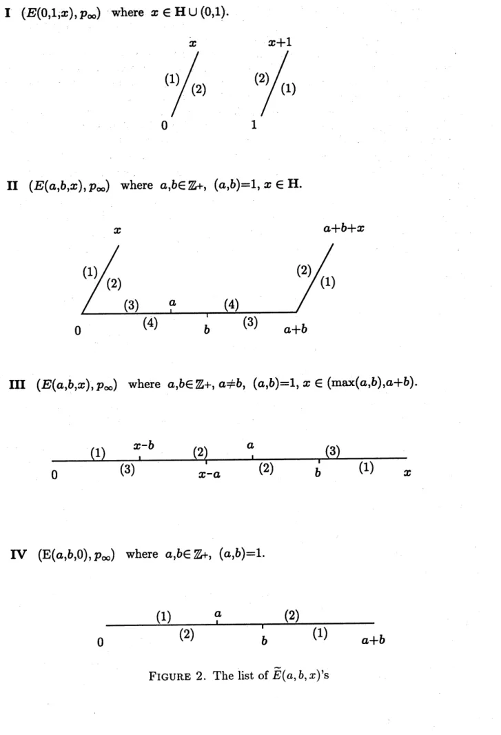
Figure

2

is a list of some once punctured elIiptic

curves

with Lagrangian sublattices denoted by $\tilde{E}(a, b, x)$ (or _$(E(a,$$b,$$x),p\infty’\Lambda 0)$) constructed from $\mathbb{C}$ by cutting along the

line segments and pasting by parallel transformations. (The numbers (1), (2),

..

. in each figure indicate pasting data

or

where to paste.) They split into the following four types,

and each

once

punctured elliptic

curve

$(E(a, b, X),p_{\infty})$ is constructed as follows:

I: (The

case

where $a=0,$ $b=1$, and $x$ is a complex number in the upper half plane

$\mathrm{H}$

or

a real number in the interval $(0,1).)$ Cut the complex plane along

$x([0,1])\cup(X([0,1])+1)$,

and paste each side $\mathrm{o}\mathrm{f}.\tau([\mathrm{o}, 1])$ and the opposite side of $(x([0,1])+1)$ by a parallel

transformation. (Igeta-construction)

II: (The

case

where $\mathit{0}$. and $b$ are relatively prime positive integers, and $x$ is

a

complex

number in the upper halfplane H.) Cut the complex plane along

I $(E(\mathrm{o},1_{X},), p\infty)$ where $x\in \mathrm{H}\cup(0,1)$

.

II $(E(a,b,X), p_{\infty})$ where $a,b\in \mathbb{Z}+,$ $(a,b)=1,$$x\in$ H.

$x$ $a+b+x$

III $(E(a,b,x), p\infty)$ where $a,b\in \mathbb{Z}+,$ $a\neq b,$ $(a,b)=1,$ $x \in(\max(a,b),a+b)$

.

rv

$(\mathrm{E}(a,b,0), p_{\infty})$ where $a,b\in \mathbb{Z}+,$ $(a,b)=1$

.

transformation and paste the upper side of (resp. ) and the lower side

of$[b, a+b]$ _(resp. $[\mathrm{o},$$b]$) by a parallel transformation.

III: (The

case

where $a$ and $b$

are

distinct relatively prime positive integers, and $x$ is a

real number such that $x \in(\max(a, b),$$a+b).)$ Cut the complex plane along $[0, x]$,

and paste the lower side of $[0, x-a]$ (resp. $[x-a,$$b],$ $1^{b,x}]$) and the upper side of

$[a, x]$ (resp. $[x-b,$$a],$ $[0,$_$x-b1$) by a parallel transformation.

IV: (The case where $a$ and $b$ are relatively prime positive integers, and $x=0.$) Cut

the complex $\mathrm{p}\mathrm{l}\mathrm{a}\mathrm{n}\mathrm{e}$

, along $[0, a+b]$ and paste the upper side of $[0, a]$ (resp.

$[a,$$a+b]$)

and the lower side of $[b, a+b]$ (resp. $[0,$$b]$) by a parallel transformation.

Note that eachelliptic

curve

constructedin thisway hasa natural Abelian differential$\omega_{0}$

induced by the differential $d\zeta$ of the standardcoordinate $\zeta$ of$\mathbb{C}$ and that the Lagrangian

sublattice $\Lambda_{0}$ of $\tilde{E}(a, b, x)$ is characterized as the kernel of the period map of $\omega_{0}$ from

$H_{1}(E(a, b, X);\mathbb{Z})$ to $\mathbb{C}$. Further, the primitive period of

$\omega_{0}$ is equal to 1 because $a$ and $b$

are

relatively prime. When $\overline{E}(a, b, x)$ is oftype I, II, or III, the set $\omega_{0}^{-1}(0)$ consists ofthe

two points$p_{0}$ and $p_{1}$ coning from the origin and the point $x$ of$\mathbb{C}$, and when $\tilde{E}(a, b, x)$ is

oftype IV, the set $\omega_{0}^{-1}(0)$ consists of the one point

$p_{0}$ coming from the origin in

$\mathbb{C}$

.

(See Figure 2.)

Our

goal in this section is to prove

Theorem 1. Foranyoncepuncturedelliptic curvewith aLagrangian sublattice $(E,p, \Lambda)$,

there exists one and only one $\tilde{E}(a, b, x)$ isomorphic to $(E,p, \Lambda)$.

We call twooncepunctured Riemann surfaces withLagrangian sublattices$(R,p, \Lambda)$ and

$(R’,p’, \Lambda/)$ isomorphic, if there exists a biholomorphic map from $R$ to $R’$ transforming $p$

to $p’$ and A into $\Lambda’$

.

In orderto prove Theorem 1 we investigate the geometry of geodesicsononcepunctured

elliptic curves having nuetlics with conical singularities induced by Abelian differentials.

Fora once punctured elliptic curve with a Lagrangian sublattice $(E,p, \Lambda)$, there exists

an

Abelian differential $\omega_{\Lambda}$, unique up to sign, in the kernel $Z_{\Lambda}$ (see [H-O1]

or

[H-O2])

such that the $\mathrm{p}_{\Gamma \mathrm{i}_{\ln}\mathrm{i}\mathrm{t}}\mathrm{i}\mathrm{v}\mathrm{e}$ period of

$\omega_{\Lambda}$ is equal to 1, because $Z_{\Lambda}$ is one-dimensional and any

non-trivial element in $Z_{\Lambda}$ has non-trivial periods. Then $\mathrm{P}\mathrm{D}[\omega_{\Lambda}]$ is an integral homology

class. Since the nletric $g_{\omega_{\Lambda}}$ on $E-p$ depends only on A in this case, we shall shortly

denote this metric by $g_{\Lambda}$. For the sanue reason we shall also use the term $\Lambda$-edge instead

of$\omega_{\Lambda}$-edge.

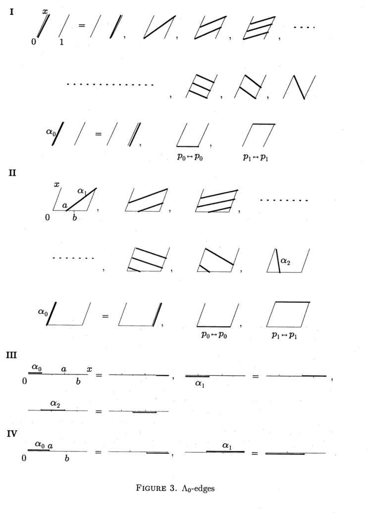
We first showthat $\tilde{E}(a, b, x)’ \mathrm{s}$ are not isomorphic to one another by studying $\Lambda_{0}$-edges.

Foreach$\overline{E}(a, b, x)$, the Abelian$\mathrm{d}\mathrm{i}\mathrm{f}\mathrm{f}\mathrm{e}\mathrm{r}\mathrm{e}\mathrm{n}\mathrm{t}\mathrm{i}\mathrm{a}1\omega_{\Lambda_{0}}$coincides with

$\omega_{0}$ uptosign. So$\Lambda_{0}$-edges

areline segments in $\mathbb{C}$ between the points of$\omega_{0}^{-1}(0)$ in each case ofFigure 2. Accordingly

we can easily obtain the following proposition.

Proposition 1. All the $\Lambda_{0}$-eclges can be described as in Figure 3

for

each $\overline{E}(a, b, x)$.

Proposition 1 implies that all the closed geodesics containing some

zeros

of$\omega_{0}$, which

consist of $\Lambda_{0}$-edges,

can

be described visually for each $\tilde{E}(a, b, x)$

.

This proposition yields

the following corollary.

Corollary 1.

_If

$(a, b, x)\neq(a’, b’, x’)$, then $\tilde{E}(a, b, x)$ is not isomorphic to $\tilde{E}(a’, b’, x’)$.

Proof.

Suppose $(E,p_{\infty}, \Lambda_{0})$ is isolnorphic to $\tilde{E}(a,.b, x)$. We shall

recover

the data_{$(a, b, x)$}

I $0^{//^{X}}$ $\int_{1}$ $=/$ $\parallel$ , $\alpha/0$ $/$

$=[$

$//$ , $p_{0}rightarrow p_{0}$ $p_{1}rightarrow p_{1}$ II $P0^{rightarrow}P^{J}0$ $p_{1}rightarrow\nu_{1}$ III $0\underline{\underline{\alpha_{0}}}$

a

_$bx=$

$\overline{\alpha_{1}}=-$

$\alpha_{2}$

$=-$

IV $\alpha_{0a}$

$=-\cdot$

, $\alpha_{1}$

$=-$

$0$ $b$

I

II

$q_{1}$ $\tau_{f\iota}$

$\mathrm{n}\mathrm{I}$

IV

FIGURE 4

We distinguish the type IV fronu others by the degeneracy of

zeros

of$\omega_{\Lambda_{0}}$, and

distin-guish the types I, II and III from each other by the properties of $\Lambda_{0}$-edges on $E$

.

Let

$\{q0, q_{1}\}$ be the set ofsingular points $\mathrm{o}\mathrm{f}/c_{\Lambda_{0}}$. (When $(E,p_{\infty}, \Lambda_{0})$ is oftype IV, let $q_{0}$ bethe unique singular point of$g_{\Lambda_{0}}.$)

When we describe all the directions of $\Lambda_{0}$-edges around

$q_{0}$,

we

obtain Figure 4 from Proposition 1. We can specify the $\Lambda_{0}$-edges $\alpha_{0},$ $\alpha_{1}$ and $\alpha_{2}$ on $E$ in Figure 4.

Note that these figures do not depend on the choice of $q_{0}$, and that there exists a $\Lambda_{0^{-}}$

edge which has the opposite direction of $\alpha_{0}$ in the case where $(E,p_{\infty’ 0}\Lambda)$ is of type I,

however in the

case

where $(E,p_{\infty}, \Lambda_{0})$ is of type II there exists noA-edge ofthis kind. We

thus specify the type of $(E,p_{\infty}, \Lambda)$. We shall orient the $\Lambda_{0}$-edges $\alpha_{0},$ $\alpha_{1}$ and $\alpha_{2}$ in Figure

4, which are also in Figure 3, $\mathrm{f}_{\Gamma \mathrm{o}\mathrm{n}1}q_{0}$ to $q_{1}$ in the case of type I, II or III.

When $(E,p_{\infty’ 0}\Lambda)$ is oftype I

or

II,

we

choose the sign of$\omega_{\Lambda_{0}}$ such that ${\rm Im} \int_{\alpha_{0}}\omega_{\Lambda_{0}}>0$

.

Then we obtain

In

case

$(E,p_{\infty}, \Lambda_{0})$ is of type II, we also obtain the following: (See Figure 3)

$a= \int_{\alpha_{0}}-\alpha_{2}\omega\Lambda 0$ ’

$b= \int_{\alpha_{1}-\alpha 0}\omega\Lambda_{0}$

.

When $(E,p_{\infty}, \Lambda_{0})$ is of type III,

we

choose the sign of$\omega_{\Lambda_{0}}$ such that $\int_{\alpha_{0}}\omega_{\Lambda_{0}}>0$

.

Then

we

obtain the following: (See Figure 3)

$a= \int_{\alpha_{0}-\alpha}2\omega_{\Lambda_{0}}$, $b= \int_{\alpha_{1}-\alpha_{2}}\omega_{\Lambda 0}$,

$x= \int_{\alpha_{0}+\alpha_{1}-\alpha_{\sim}},\omega_{\Lambda_{0}}$

.

When $(E,p_{\infty}, \Lambda_{0})$ is of type IV, we obtain the following: (See Figure 3)

$a=| \int_{\alpha_{0}}\omega_{\Lambda_{0}}|$, $b=| \int_{\alpha_{1}}\omega_{\Lambda_{0}}|$.

Wethereby

recover

the data $(a, b, x)$ from $(E,p_{\infty}, \Lambda_{0})$ in any

case.

Hencethis corollary

follows. $\square$

Corollary 1 inuplies the uniqueness in Theorem 1. In order to finish

our

proofof The-oreml,

we

next show the completeness; for a $\mathrm{g}\underline{\mathrm{i}\mathrm{v}}\mathrm{e}\mathrm{n}$ once punctured elliptic

curve

with

a

Lagrangian sublattice $(E,p, \Lambda)$, there exists an$E(a, b, x)$ which is isomorphic to $(E,p, \Lambda)$

.

Let $\gamma$ be an oriented loop or map from

$S^{1}$ to $E$ representing a generator of A. The

Abelian differential $\omega_{\Lambda}$ is exact on $E-\gamma(S^{1})$ because the integral of $\omega_{\Lambda}$ along a loop $\alpha$

equals zero if and only if $\alpha \mathrm{r}\mathrm{e}_{1^{)\mathrm{r}\mathrm{e}\mathrm{S}}}\mathrm{e}\mathrm{n}\mathrm{t}\mathrm{S}$ a homology class whose intersection number with

the homology class $[\gamma]$ equals zero. When we denote by $||\gamma||$ the length of

$\gamma$ with respect

to the metric $g_{\Lambda}$, it is verified fronl the followingtwo facts (1), (2) that there exists

a

loop

representing a generator ofA which has the smallest length

among

such loops, and that the loop consists ofA-edges. We shall call

a

loop consisting of A-edges

a

$\Lambda$-edge-loop.

(1): For any loop $\alpha$ on $E$, thereexists a$\Lambda$-edge-loop $\alpha’$ consisting ofA-edges such that

$\alpha’$ is homotopic to

$\alpha$ and $||\alpha’||\leq||\alpha||$.

(2): For any positive nunuber $r$, there exist at most finitely many $\Lambda$-edge-loops with

length smaller than $r$.

We

can

show that fact (1) follows thisway: we first approximate$\alpha$ by

a

polygonal loop,

and then

we

reduce the nunlber ofvertices which donot lie

on

$\omega_{\Lambda}(0)$

.

On

the other hand, for a positive number $r$, it is obvious that there exist at most finitely many A-edges with

length smaller than $r$, and then the fact (2) follows.

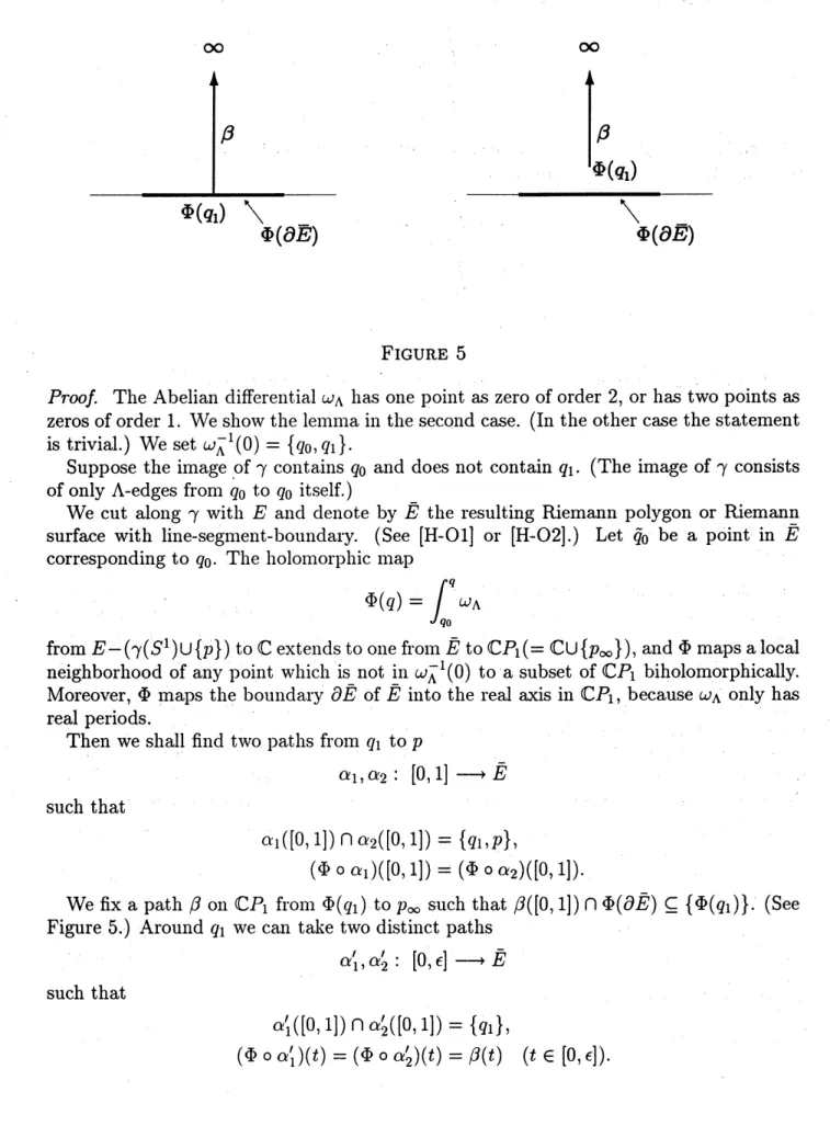
Lemma 1. The image

_of

an oriented$\Lambda$-edge-loop

$\gamma$ representing agenerator

of

A contains

$\infty$ $\infty$

$|_{\sqrt}\Phi(q_{1})$

$\backslash _{\Phi(\partial\overline{E})}$

FIGURE 5

Proof.

The Abelian differential $\omega_{\Lambda}$ has

one

point as zero of order 2, or has twopoints

as

zeros

oforder 1. We show the lemma in the second

case.

(In the other

case

the statement

is trivial.) We set $\omega_{\Lambda}^{-1}(0)=\{q_{0}, q_{1}\}$.

Suppose the image of $\gamma$ contains $q_{0}$ and does not contain $q_{1}$

.

(The image of$\gamma$ consists

of only A-edges from $q_{0}$ to $q_{0}$ itself.)

We cut along $\gamma$ with $E$ and denote by

$\overline{E}$ the resulting Riemann polygon or Riemann

surface with $1\mathrm{i}\mathrm{n}\mathrm{e}- \mathrm{s}\mathrm{e}\mathrm{g}\mathrm{m}\mathrm{e}\mathrm{n}\mathrm{t}-\mathrm{b}_{0}\mathrm{u}\mathrm{n}\mathrm{d}\mathrm{a}\mathrm{r}\mathrm{y}$ . (See [H-O1] or [H-O2].) Let $\tilde{q}_{0}$ be a point in

$\overline{E}$

corresponding to $q_{0}$. The holomorphic nuap

$\Phi(q)=\int_{q_{0}}^{q}\omega_{\Lambda}$

from$E-(\gamma(s^{1})\cup\{p\})$ to$\mathbb{C}$ extends toonefrom $\overline{E}$to

$\mathbb{C}P_{1}(=\mathbb{C}\cup\{p_{\infty}\})$, and $\Phi$maps alocal

neighborhood of any point which is not in $\omega_{\Lambda}^{-1}(0)$ to a subset of $\mathbb{C}P_{1}$ biholomorphically.

Moreover, $\Phi$ maps the boundary $\partial\overline{E}$ of $\overline{E}$ into the real axis in $\mathbb{C}P_{1}$, because

$\omega_{\Lambda}$ only has

real periods. _.

Then we shall find two paths from $q_{1}$ to $p$

$\alpha_{1},$ $\alpha_{2}$

:

$[0,1]arrow\overline{E}$

such that

$\alpha_{1([1]}\mathrm{o},)\mathrm{n}\alpha 2(10,1])=\{q1,p\}$,

$(\Phi 0\alpha_{1})([0,11)=(\Phi 0\alpha_{2})([0,1])$. We fix apath $\beta$ on $\mathbb{C}P_{1}$ fronl $\Phi(q1)$ to

$p_{\infty}$ such that $\beta([0,1])\cap\Phi(\partial\overline{E})\subseteq\{\Phi(q_{1})\}$. (See Figure 5.) Around $q_{1}$ we can take two distinct paths

$\alpha_{1}’,$$\alpha_{2}’$

:

$[0, \epsilon]arrow\overline{E}$

such that

$\alpha_{1}’([\mathrm{o}, 1])\cap\alpha_{2}/(10,1])=\{q1\}$,

Since $\Phi$ is a local biholomorphic map except

$q_{0},$ $q_{1}$,

we

obtain the desired paths $\alpha_{1},$ $\alpha_{2}$

as

the pull-back of $\beta$ by $\Phi$ which coincide

near

$q_{1}$ with $\alpha_{1}’,$ $\alpha_{2}’$ respectively. Meanwhile,

the map $\Phi$ is bihololnorphic alound

$p$. This is acontradiction.

We recall three well-known facts about simple loops

on

elliptic

curves.

Fact (1): _{The holnology class represented by asimple loop is trivial}

_or

_primitive. Fact (2): If $\gamma$ and $\gamma’$ are simple loops such that their homology classes

$[\gamma],$ $[\gamma’]$ are

primitive and their intersection number $[\gamma]\cdot[\gamma’]$ is equal to zero, then $[\gamma]=\pm[\gamma]’$

.

Fact (3): If $\gamma$ and $\gamma’$ are simple loops such that their intersection number is equal to

$\pm 1$, then the pair _{$([\gamma], [\gamma’])$} is a basis of

$H_{1}(E;\mathbb{Z})$

.

Since the integral value of $\omega_{\Lambda}$ along any A-edge does not vanish, the following lemma

follows from Fact (2) and the definition of A-edge immediately, and we omit its proof.

(Note that two distinct parallel A-edges have no

common

points except the points in

$\omega_{\Lambda}^{-1}(\mathrm{o}).)$

Lemma 2. Suppose $\omega_{\Lambda}^{-1}(0)$ consists

of

two distinct points

$q_{0},$ $q_{1}$

.

If

$\gamma_{1}$ (resp. $\gamma_{2}$) is a

$A$-edge

from

$q_{0}$ to $q_{0}$

itself

(resp. $q_{1}$ to $q_{1}$ itself), then $[\gamma_{1}]=\pm[\gamma_{2}]\in H_{1}(E;\mathbb{Z})$.

Let $\gamma_{(0)}$ beanoriented$\Lambda$-edge-looprepresenting agenerator ofAand havingthe smallest

length. When we consider $\gamma_{(0)}$ as an ordered set of oriented A-edges, we may obtain

another loop $\gamma_{(0)}’$ representing the same homology class by reordering the oriented $\Lambda-$

edges suitably. (We assunle that each A-edge inherits its orientation from $\gamma_{(0)}.$) We

obtain the following lennma about $\gamma_{(0)}$.

Lemma

3. The $im$age

of

$\gamma_{(0)}$ consists

of

$\Lambda$-edges which have no intersection with

one

another except$\omega^{-1}(0)$.

Proof.

When $\omega_{\Lambda}$ has a zero of order 2, the

$\mathrm{l}\mathrm{e}\mathrm{n}\mathrm{l}\mathrm{n}\mathrm{l}\mathrm{a}$is immediate

because all the A-edges

are parallel. We thus consider the case where $\omega_{\Lambda}$ has two points _{$q_{0},$} $q_{1}$ as

zeros.

We consider $\gamma_{(0)}$ as an ordered set $(\gamma_{1}, \gamma_{2}, \ldots , \gamma_{l})$ of oriented A-edges. Suppose A-edges

$\gamma_{i}$ and $\gamma_{j}(1\leq i\leq j\leq l)$ have an intersection at a point $q\not\in\omega_{\Lambda}^{-1}(0)$. Then both

$\gamma_{i}$ and

$\gamma_{j}$ are A-edges between $q_{0}$ and $q_{1}$, and they intersect each other transversely. We prepare paths $\gamma_{i}’$ and

$\gamma_{j}’$ modifying $\gamma_{i}$ and $\gamma_{j}$ around $q$ as in Figure

6.

We replace $\gamma_{i},$ $\gamma_{j}$ with $\gamma_{i}’,$ $\gamma_{j}’\mathrm{r}\mathrm{e}\mathrm{s}_{\mathrm{P}^{\mathrm{e}\mathrm{c}\mathrm{t}\mathrm{i}}}\mathrm{V}\mathrm{e}\mathrm{l}\mathrm{y}$, and set

$\gamma_{(0)}’=(\gamma 1, \ldots, \gamma i, \ldots, \gamma j, \ldots, \gamma l)$

.

Then the cycle $\gamma_{(0)}’$ represents the homology class $[\gamma_{(0)}]$.

In the

case

(1)

or

(2),

we can

consider $\gamma_{(0)}’$

as

a

loop, and the length $||\gamma_{(0)}’||$ is smaller

than $||\gamma_{(0)}||$

.

This contradicts the definition of

$\gamma_{(0)}$

.

In the case (3) or (4), it is necessary to reorder the elements of $\gamma_{(0)}’$. Ifthere still exist

A-edges between $q_{0}$ and $q_{1}$ in $\gamma_{(0)}’$, then it is easy to obtain a loop by reordering the

paths and loops $\{\gamma_{1}, \ldots , \gamma_{i’\ldots,\gamma_{j}}’’, \ldots, \gamma_{k}\}$ whose length is smaller than $||\gamma_{(0)}||$. This also

contradicts the definition of$\gamma_{(0)}$. Ifthereexist no more A-edges between $q_{0}$ and $q_{1}$ in $\gamma_{(0)}’$,

we

further replace the loop $\gamma_{i}’$ by A-edges from

$q_{0}$ to $q_{0}$ itself, the loop $\gamma_{j}’$ by A-edges from

$q_{1}$ to $q_{1}$ itselfpreserving the homology class. Moreover, byusing Lemma 2,

we can

replace all the A-edges from $q_{1}$ to $q_{1}$ itself by A-edges from $q_{0}$ to $q_{0}$ preserving the homology class.

(1) (2)

$a_{\tau}$ $a$, $O\tau$ $q_{1}$

(3) (4)

FIGURE 6

Then we obtain a cycle $\mathrm{r}\mathrm{e}\mathrm{p}\mathrm{r}\mathrm{e}\mathrm{S}\mathrm{e}\mathrm{n}\mathrm{t}\mathrm{i}_{1\mathrm{l}}\mathrm{g}$ the cohomology class $1^{\gamma(0)}$], and consisting of only A-edges from $q_{0}$ to $q_{0}$ itself. This cycle

can

be considered

as

a loop, and this contradicts

Lemma 1.

Proof of

Theorem 3. Let $\gamma_{(0)}$ be an oriented

$\Lambda$-edge-loop representing a generator ofA

and having the smallest length

as

before. We describe $\gamma(0)$

as an

ordered set of oriented

A-edges;

$\gamma_{(0)}=(\gamma_{1}, \ldots, \gamma l)$

.

We first consider thecase where $\omega_{\Lambda}^{-1}(0)$ consistsof only

one

point $q_{0}$. Inthis case, each element $\gamma_{k}$ of $\gamma_{(0)}$ is

an

oriented sinuple loop

on

$E$, and the integral of$\omega_{\Lambda}$ along $\gamma_{k}$ is

a

non-zero

integer. Hence it follows from Fact (2) that $\gamma_{k}$ represents a primitive class in

$H_{1}(E;\mathbb{Z})$

.

We shall choose the sign of$\omega_{\Lambda}$ such that

$\int_{\gamma_{1}}\omega_{\Lambda}>0$

.

Since

the integral of$\omega_{\Lambda}$ along $\gamma(0)$ is equal to zero, we may further

assume

by reordering

$\int_{\gamma_{\sim}},\omega_{\Lambda}<0$

.

The loops$\gamma_{1}\mathrm{a}\mathrm{n}\mathrm{d}-\gamma 2$ represent different homologyclasses, because

$\gamma_{(0)}$ has the smallest length.

On

the other hand, they intersect each other only at $q_{0}$. Hence from Facts (1) and (2) it follows that their intersection nunuber at $q_{0}$ is equal to 1 or-l and that the pair $([\gamma_{1}], [\gamma_{2}])$ is a basis of$H_{1}(E;\mathbb{Z})$.

(i) (ii)

FIGURE 7

Cut $E$ along $\gamma_{1}$ and $\gamma_{-}$” and denote by

$\overline{E}$ the resulting Riemann polygon. In each case

in Figure 7, by choosing apoint $\tilde{q}_{0}$ in $\partial\overline{E}$

suitably (see Figure 7),

we

obtain aholomorphic

map $\Phi$ from $\overline{E}$ to $\mathbb{C}P_{1}$:

$\Phi(q)=\int_{q)}^{q}\omega_{\Lambda}$.

In

case

(i), set

$a= \int_{\gamma_{1}}\omega_{\Lambda}$,

$b=- \int_{\gamma_{2}}\omega_{\Lambda}$.

In case (ii), set

$o=- \int_{\gamma}\underline,\omega_{\Lambda}$,

$b= \int_{\gamma_{1}}\omega_{\Lambda}$

.

Then the integers $a$ and $b$

are

relatively $\mathrm{p}_{\Gamma \mathrm{i}\mathrm{n}}\mathrm{u}\mathrm{e}$ because the pair $([\gamma_{1}], [\gamma_{2}])$ is

a

$\mathrm{b}\mathrm{a}s$is of

$H_{1}(E;\mathbb{Z})$, and then $\Phi$ gives rise to an isomorphism between $(E,p, \Lambda)$ and $\tilde{E}(a, b, \mathrm{o})$

.

We next consider the other

case:

$\omega_{\Lambda}^{-1}(0)$ consists of two distinct points $q_{0}$ and $q_{1}$

.

In

this case, from Lenlma 1 there exists at least one A-edge from $q_{0}$ to $q_{1}$ and at least

one

A-edge from $q_{1}$ to $q_{0}$ in $\gamma_{(0)}$

.

We may

assume

that $\gamma_{1}$ is a A-edge from $q_{0}$ to $q_{1}$

.

We may

further assume from Lemnua 2 that $\gamma_{(0)}$ does not contain A-edges from $q_{1}$ to $q_{1}$ itself.

$\int_{\gamma}.\cdot\omega_{\Lambda}=-\int_{\gamma_{1}}\omega_{\Lambda}$. Because $\gamma(0)$ has the smallest length, the simple loop

$(\gamma_{1}, \gamma_{i})$ is non-trivial, and hence primitive (Fact (1)). Therefore we obtain $\gamma_{(0)}=(\gamma_{1}, \gamma_{i})$

.

(Note that aloop $\gamma$ representing

a

generator of A is

characterized

by two properties;

one

is that $\gamma$ represents

a

primitive

homology class, and the other is that the integral of$\omega_{\Lambda}$ along$\gamma$ vanishes.)

Cut $E$ along $\gamma_{1}$ and $\gamma_{i}$, denote by

$\overline{E}$

the resulting Riemann polygon, and set the

signature of$\omega_{\Lambda}$ such that

${\rm Im}( \int_{\gamma 1}\omega\Lambda)>0$ or $\int_{\gamma_{1}}\omega_{\Lambda}>0$

.

By choosing

a

point $\tilde{q}_{0}$ in

$\partial\overline{E}$suitably, weobtain a holomorphic map $\Phi$ from $\overline{E}$ to $\mathbb{C}P_{1}$:

$\Phi(q)=\int_{r}^{q}\omega_{\Lambda}$

.

If

we

set

$x= \int_{\gamma_{1}}\omega_{\Lambda}$,

then $\Phi$ gives rise to an $\mathrm{i}_{\mathrm{S}\mathrm{o}\mathrm{m}}\mathrm{o}\Gamma \mathrm{p}\mathrm{h}\mathrm{i}\mathrm{s}\mathrm{n}1$ between$(E,p, \Lambda)$ and $\overline{E}(0,1, x)$. (Igeta-construction) (ii) Suppose

$\int_{\gamma}.\cdot\omega_{\Lambda}\neq-\int_{\gamma_{1}}\omega_{\Lambda}$

for any $\gamma_{i}$, A-edge fronu $q_{1}$ to $q_{0}$ in $\gamma(0)$.

(ii-a) When the integral of$\omega_{\Lambda}$ along $\gamma_{1}$ is not areal number, we choose the sign of$\omega_{\Lambda}$

such that

$\mathrm{I}\mathrm{n}1(\int_{\gamma}1\omega\Lambda)>0$.

We may

assume

without loss of generality that there exists a A-edge $\gamma_{i}$ from $q_{1}$ to $q_{0}$ in $\gamma_{(0)}$ such that the integral of$\omega_{\Lambda}$ along$\gamma_{1}+\gamma_{i}$ is apositive integer. We mayfurther assume

by reordering that the integral of$\omega_{\Lambda}$ along $\gamma_{1}+\gamma_{2}$ is minimal among such

$\gamma_{i}’ \mathrm{s}$.

$\int_{\gamma_{1}+\gamma:}\omega_{\Lambda}\geq\int_{\gamma_{1}+\gamma 2}\omega_{\Lambda}\geq 0$

Since

the integralof$\omega_{\Lambda}$ along $\gamma_{(0)}$ vanishes,

we see

from the inequality above that there

occur the following two cases:

1: There exists in $\gamma_{(0)}$ a A-edge $\gamma_{j}$ from $q_{0}$ to $q_{0}$ such that

$\int_{\gamma \mathrm{j}}\omega_{\Lambda}<0$

.

2: Thereexist in $\gamma_{(0)}$ A-edges $\gamma_{\mu}$ and $\gamma_{\nu}$ ($\gamma_{\mu}$ is from $q_{0}$ to $q_{1},$ $\gamma_{\nu}$ from $q_{1}$ to $q_{0}$) such that

(1)

(2)

$\Phi(\overline{E})=$

FIGURE 8

Suppose the following two inequalities hold for any$\gamma_{\mu}$ from $q_{0}$ to $q_{1}$ and for any $\gamma_{\nu}$ from

$q_{1}$ to $q_{0}$.

$\int_{\gamma+\gamma_{\mu}}\underline,\omega_{\Lambda}\geq 0$, $\int_{\gamma_{1}+\gamma_{\nu}}\omega_{\Lambda}\geq 0$

Then we obtain the following inequality $\mathrm{f}\mathrm{r}\mathrm{o}\ln$ the second inequality above and the choice of$\gamma_{2}$.

$\int_{\gamma_{1}+\gamma_{\nu}}\omega_{\Lambda}\geq\int_{\gamma_{1}+\gamma_{2}}\omega_{\Lambda}$

Furthermore

we

obtain the following inequality, and this is a contradiction.

$\int_{\gamma_{\mu}+\gamma_{\nu}}\omega_{\Lambda}=\int_{\gamma_{\mu}+\gamma}\underline,\omega_{\Lambda}-\int_{\gamma_{\vee}+\gamma 1},\omega_{\Lambda}+\int_{\gamma_{1}+\gamma_{\nu}}\gamma\Lambda$

$\geq\int_{\gamma_{l^{l}}\gamma_{-}}+\cdot\omega_{\Lambda}$

$\geq 0$.

Therefore the following three cases occur:

(1) there is $\gamma_{j}$ from $q_{0}$ to $q_{1}$ such that

$\int_{\gamma_{1}+\gamma j}\omega_{\Lambda}<0$

.

(3) there is $\gamma_{j}$ from $q_{0}$ to $q_{0}$ such that

$\int_{\gamma_{j}}\omega_{\Lambda}<0$

.

The figures on the left-hand side of Figure 8 indicate the images of $\gamma_{1},$ $\gamma_{2}$, and $\gamma_{j}$ by

the integral of$\omega_{\Lambda}$ in each case above.

In the case (1), we shall show that the homology classes represented by the simple

loops $(\gamma_{1},\gamma_{2})$ and $(\gamma_{j}, \gamma_{2})$ form

a

$\mathrm{b}\mathrm{a}s$is of $H_{1}(E;\mathbb{Z})$; If the homology classes $[(\gamma_{1},\gamma_{2})]$ and

$-[(\gamma_{j}, \gamma_{2})]$ represent the

same

homology class, then we get a loop $\gamma_{(0)}’$ representing a

generator of A by removing $\gamma_{1},$ $\gamma_{2}$, and $\gamma_{j}$ from $\gamma_{(0)}$ and placing $-\gamma_{2}$ instead, and $\gamma_{(0)}’$ is shorter than $\gamma_{(0)}$

.

This is a contradiction. Hence fronu Facts (1) and (2) it follows that the intersection $\mathrm{n}\mathrm{u}\mathrm{n}\mathrm{l}\mathrm{l}\supset \mathrm{e}\mathrm{r}[(\gamma_{1}, \gamma_{2})]\cdot[(\gamma_{j}, \gamma 2)]$ is not equal to

zero.

On the other hand,

$(\gamma_{1},\gamma_{2})$ intersects $(\gamma_{j}, \gamma_{2})$ only at $\gamma_{2}$

.

Therefore the pair $([(\gamma 1, \gamma 2)], [(\gamma_{j}, \gamma_{2})])$ is a basis of

$H_{1}(E;\mathbb{Z})$

.

In the

same

way, weobtain the fact that the pair $([(\gamma_{1}, \gamma_{2})], [(\gamma_{1}, \gamma j)])$ is

a

basis

of$H_{1}(E;\mathbb{Z})$ in the

case

(2), and that the pair $([(\gamma 1, \gamma_{2})], [\gamma_{j}])$ is a basis of$H_{1}(E;\mathbb{Z})$ in the

case

(3).

Cut $E$ along $\gamma_{1},$ $\gamma_{2}$, and $\gamma_{j}$ in each case, and then denote by

$\overline{E}$ the resulting Riemann

polygon. We obtain aholomorphic nuap $\Phi$ from $\overline{E}$ to $\mathbb{C}P_{1}$

$\Phi(q)=\int_{\mathfrak{g})}^{q}\omega_{\Lambda}$

when we choose abase point $\tilde{q}_{0}$ in $\overline{E}$

, because we obtain a basis of$H_{1}(E;\mathbb{Z})$ from $\gamma_{1},$ $\gamma_{2}$,

and $\gamma_{j}$

.

In the

case

(1), let $\tilde{q}_{0}$ be the point in the boundary

$\partial\overline{E}$

which is the initial point of$\gamma_{1}$

and is also the end point of$\gamma_{2}$. Then we get the image

$\Phi(\overline{E})$

as

in the middle figure in

Figure 8. It is now easy to nlodify $\overline{E}$ by cutting and pasting from $\Phi(\overline{E})$ such that we can

obtain a Riemann polygon of type II. (See Figure 8.) Note that $a’$ and $b’$ are relatively

prime integers where $b’$ is the integral of$\omega_{\Lambda}$ along $(\gamma_{j}, \gamma_{2})$

.

In the similar way, we obtain a Rielnann polygon of type II in the cases (2) and (3),

and omit the explanation.

(ii-b) When the integral of $\omega_{\Lambda}$ along $\gamma_{1}$ is a real number, there also exists

an

element $\gamma_{j}$ in $\gamma(0)$ different from $\gamma_{1}$ and $\gamma_{2}$

.

We obtain the fact that $\gamma_{j}$ joins $q_{0}$ with $q_{1}$ as follows: Suppose $\gamma_{j}$ is

a

A-edge from $q_{0}$ to $q_{0}$ itself. We may

assume

$( \int_{\gamma 1+\gamma_{\sim}},\omega_{\Lambda})\cdot(\int_{\gamma j}\omega\Lambda)<0$

.

The simple loop $\gamma_{j}$ intersects the simple loop

$(\gamma_{1}, \gamma_{2})$ at $q_{0}$ with

intersection

number

zero

because the directions of$\gamma_{1},$ $\gamma_{2}$, and $\gamma_{j}$ can be described

as

in the following figure. Hence

it follows from Fact (2) that the $\mathrm{h}_{\mathrm{o}\mathrm{n}\mathrm{l}\mathrm{O}}\mathrm{l}\mathrm{o}\mathrm{g}\mathrm{y}$ class $[\gamma_{1}+\gamma_{2}+\gamma_{j}]$ vanishes. This contradicts

the definition of$\gamma_{(0)}$

.

Now

we

may

assume

that $\gamma_{j}$ is an edge from $q_{0}$ to $q_{1}$

.

Then the two homology classes

[$(\gamma_{1},\gamma 2)1$ and $[(\gamma j, \gamma_{2})]$ fornu a basis of $H_{1}(E;\mathbb{Z})$. We can also describe the directions of

(1) (2)

$||1^{\cdot}\mathrm{t}\mathrm{I}\iota_{---}\prime^{\frac{j_{\mathrm{z}}\overline{\int}^{2}\prime--\backslash }{\backslash q_{0}\gamma\sim\prime}---}\gamma--- 1^{--\backslash }--\backslash ---|11l|’\sim---.---\cdot!\mathrm{T}_{l}^{l}---\wedge|1$

around

$q_{0}$

around

$q_{1}$

(3) (4)

$l\iota^{\prime^{\frac{\mathrm{j}\backslash \overline{\mathrm{r}}^{2^{--}}\prime\backslash }{q_{0}\gamma\sim\prime}-}}1|1_{--}\gamma--,---..-\vee-\backslash -- 1---\backslash ||\mathrm{l}1\iota’----\cdot---\mathrm{T}^{1},-|1|1$

.

$|\gamma^{\frac{\backslash \backslash q_{0}\gamma\sim}{2\mathrm{b}_{\mathrm{j}}’\backslash _{---}}-}l\iota_{-}\mathrm{I}’---,---.- 1---’--\cdot\perp’|1^{\backslash }..|||1|---\sim{}^{\mathrm{t}}\iota|.|$

.

(5) (6)

$\gamma,1\mathrm{I}\mathrm{l}\mathrm{I}11_{--}\prime^{\frac{j_{r\backslash }\overline{q}0\gamma}{\backslash \mathrm{b}_{2}\backslash _{---}}}---_{J}-’.\cdot.\cdot.1---\iota----\perp_{\mathrm{I}}\vee l||\mathrm{t}|’\backslash --- 1$

.

FIGURE

9

Cut $E$ along $\gamma_{1},$ $\gamma_{2}$, and $\gamma_{j}$, and denote by

$\overline{E}$ the resulting Riemann polygon. We

choose the point $\tilde{q}_{0}$ at the vertex

on

$\partial\overline{E}$ where the boundary is smooth. (See Figure 9.)

We ’

$\mathrm{c}$hoose the sign of$\omega_{\Lambda}$ such that $\Phi \mathrm{n}\mathrm{u}\mathrm{a}_{\mathrm{P}^{\mathrm{S}}}$ each point to a positive number

around

$\tilde{q}_{0}$

.

Then the map $\Phi$ gives rise to an isomorphism between $(E,p, \Lambda)$ and $\tilde{E}(a, b, x)$ oftype III for

some

$(a, b, x)$. We have completed the proof of Theorem 1.

We denote by $\mathcal{M}\mathcal{L}_{1,1}$ the set ofonce punctured elliptic

curves

with Lagrangian

sublat-tices;

$\mathcal{M}\mathcal{L}_{1,1}=\{\tilde{E}(a, b, x)\}$

.

We will consider the complex structure of$\mathcal{M}\mathcal{L}_{1,1}$ in the next section. 3. COMPLEX STRUCTURE OF $\mathcal{M}\mathcal{L}_{1,1}$

When we consider the forgetful nuap from the set $\mathcal{M}L_{1,1}$ of

once

punctured elliptic

curves

with Lagrangian sublattices to the

moduli

space $\mathcal{M}_{1,1}$ of

once punctured

elliptic

curves, it should be a $\mathrm{h}\mathrm{o}\mathrm{l}\mathrm{o}\mathrm{n}\mathrm{l}\mathrm{o}\mathrm{r}\mathrm{p}\mathrm{h}\mathrm{i}_{\mathrm{C}\mathrm{n}\mathrm{u}}\mathrm{a}\mathrm{P};\mathcal{M}\mathcal{L}_{1,1}$ should be a complex $V$-manifold whose

complex structure is

induced

from $\mathcal{M}_{1,1}$ by the forgetful map.

We consider the conuplex structure of $\mathcal{M}\mathcal{L}_{1,1}$ by using the description in Theorem 1: We give

a

local coordinate of $\mathcal{M}\mathcal{L}_{1,1}$

around

each

once punctured

elliptic

curve

with

$arrow J\iota$ $j_{-t}arrow$

$\mathbb{C}-s_{t}$ $U_{|t|}$ $\mathbb{C}-s_{-t}$

FIGURE

10

a Lagrangian sublattice $\tilde{E}(a, b, x)$. For this purpose we first prepare two methods of

deforming complex structures of Riemann surfaces.

$\mathrm{S}\mathrm{e}\mathrm{t}\mathrm{L}\mathrm{e}\mathrm{t}t$ be

$\mathrm{a}$ complex number

$\mathrm{a}\mathrm{n}\mathrm{d}\mathrm{l}\mathrm{e}\mathrm{t}-,s_{t}$ be the line segment between

$\sqrt{t}$ and $-\sqrt{t}$in $\mathbb{C}$.

$U_{|t|}:=\{z\in \mathbb{C};|z|>|\sqrt{t}|\}$. Then the following nuap $J_{t}$ is biholomorphic:

$J_{t}$

:

$U_{|t}| \ni Z-\frac{1}{2}(z+\frac{t}{z})\in \mathbb{C}-s_{\iota}$.

Hence we obtain a biholomorphic map $J_{t}\mathrm{o}J_{-}^{-1}t$ from $\mathbb{C}-s_{-t}$ to $\mathbb{C}-s_{t}$

.

Note that the

map $J_{tt}\mathrm{o}J_{-}^{-1}$ is parametrized by $t\mathrm{h}\mathrm{o}1_{\mathrm{o}\mathrm{n}\mathrm{l}\mathrm{O}\Gamma}\mathrm{p}\mathrm{h}\mathrm{i}\mathrm{c}\mathrm{a}\mathrm{l}\mathrm{l}\mathrm{y}$. (See Figure 10.)

On the other hand, let $s_{1}’$ be the union oftwo line segments; the line segment from $0$

to 1 and the line segnuent from $0$ to $e^{\tilde{\frac{}{3}}\pi i}’$

.

We denote by $IC$ the biholomorphic map from

$U_{1}=\{z\in \mathbb{C};|z|>1\}$ to $\mathbb{C}-s_{1}’$ such that $K(1)=0$

.

(There exists uniquely such a

biholomorphic map due to Riemann’s mapping theorem.) Let $t$ be a complex number as above. We also denote by $t$ the automorphism of$\mathbb{C}$ defined by multiplication by $t$. Set

$s_{t}’=t(s_{1}’)$.

Then $I\zeta_{t}:=t\mathrm{o}K\mathrm{o}t^{-}1$ is a $\mathrm{b}\mathrm{i}\mathrm{h}\mathrm{o}1_{0}\mathrm{n}\mathrm{u}\mathrm{o}\mathrm{r}\mathrm{p}\mathrm{h}\mathrm{i}_{\mathrm{C}}$ map from _{$U_{|t|}$} to $\mathbb{C}-s_{t}’$. The map $I\{_{t}$ is

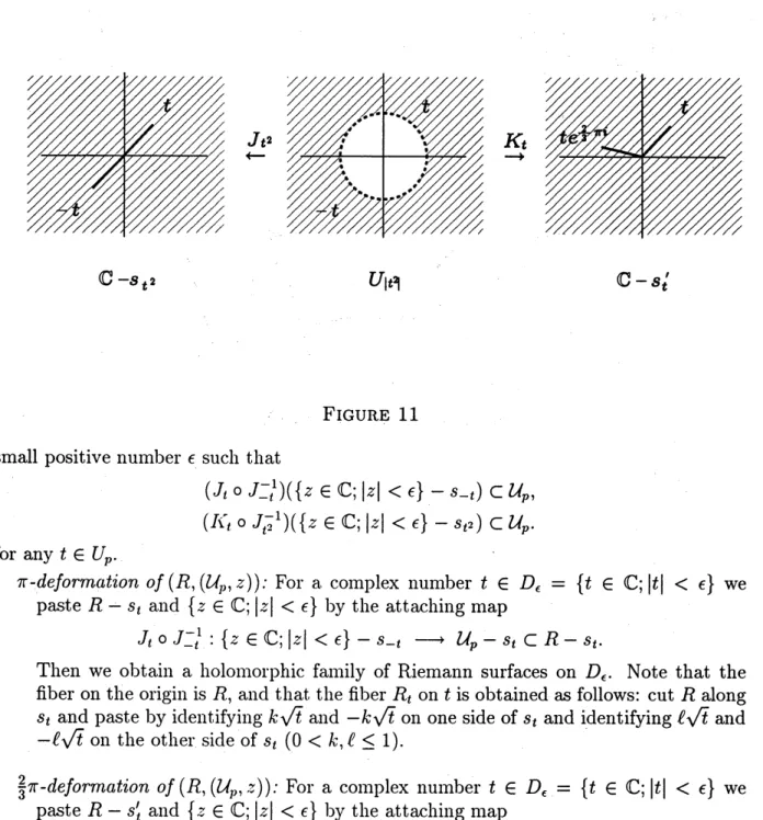
parametrized by $t$ holonlorphically even at $t=0$. We consider the biholomorphic map

$I\zeta_{t^{\mathrm{O}}}J_{l^{2}}^{-}1$ from $\mathbb{C}-s_{t^{2}}$ to $\mathbb{C}-s_{t}’$, which is also parametrized by $t$ holomorphically. (See Figure 11.)

Let $p$ be a point on a Rienlann surface $R$, and fix a local coordinate $z$ : $\mathcal{U}_{p}arrow \mathbb{C}$

$(z(p)=0)$ around $p$

.

The subset $\mathcal{U}_{p}$ of $R$ is also regarded as a subset of$\mathbb{C}$, and then both

$arrow J_{t^{2}}$ $K_{t}arrow$

$\mathbb{C}-s_{t^{2}}$ $U_{|t1}$ $\mathbb{C}-s_{t}’$

FIGURE 11

small positive number $\epsilon$ such that

$(J_{t}\mathrm{o}J_{-}^{-}1)t(\{Z\in \mathbb{C};|z|<\epsilon\}-s_{-1})\subset \mathcal{U}_{p}$, $(I\mathrm{i}_{t}’\mathrm{O}J^{-}2)t(1\{Z\in \mathbb{C};|z|<\epsilon\}-s_{t}2)\subset \mathcal{U}_{p}$.

for any $t\in U_{p}$.

$\pi$

-deformation of

$(R, (u_{p}, z))$: For a complex number _{$t\in D_{\epsilon}=\{t\in \mathbb{C};|t|<\epsilon\}$} we

paste $R-s_{t}$ and $\{z\in \mathbb{C};|z|<\epsilon\}$ by the attaching map

$J_{t}\mathrm{o}J_{-t}^{-1}$ : _{$\{_{Z\in}\mathbb{C};|z|<\epsilon\}-S-tarrow \mathcal{U}_{p}-s_{t}\subset R-s_{t}$}

.

Then we obtain a $\mathrm{h}\mathrm{o}\mathrm{l}\mathrm{o}\mathrm{m}\mathrm{o}\mathrm{l}\mathrm{P}^{\mathrm{h}\mathrm{i}_{\mathrm{C}}}$ family of Riemann surfaces on $D_{\epsilon}$. Note that the

fiberon the origin is $R$, and that the fiber $R_{t}$ on $t$ is obtained as follows: cut _$R$ along

$s_{t}$ and paste by identifying $k\sqrt{t}\mathrm{a}\mathrm{n}\mathrm{d}-k\sqrt{t}$on one side of$s_{t}$ and identifying$\ell\sqrt{t}$ and

$-l\sqrt{t}$ on the other side of _{$s_{t}(0<k, \ell\leq 1)$}.

$\frac{2}{3}\pi$

-deformation of

$(R, (\mathcal{U}_{p}, z))$: For a complex number $t\in D_{\epsilon}=\{t\in \mathbb{C};|t|<\epsilon\}$ we

paste $R-s_{t}’$ and $\{\approx\in \mathbb{C};|z|<\epsilon\}$ by the attaching map

$I\zeta_{t}\mathrm{o}J_{t\underline’}^{-1}$

:

$\{_{\mathcal{Z}\in \mathbb{C};}|z|<\epsilon\}-s_{t}2arrow \mathcal{U}_{P^{-S’\subset}}R-tS’t$.

Then we obtain a $\mathrm{h}\mathrm{o}1_{01\mathrm{n}\mathrm{o}}\mathrm{r}\mathrm{p}\mathrm{h}\mathrm{i}\mathrm{c}$ fanlily of Riemann surfaces on $D_{\epsilon}$. Note that the

fiber on the origin is $R$, and that the fiber $R_{t}$ on$t$is obtained asfollows: cut $R$along

$s_{t}’$ and paste by identifying $kt$ and $kte^{\tilde{\frac{}{3}}\pi i}$

’

on one side of $s_{t}’$ and identifying $\ell t$ and

$-\ell te^{\frac{2}{3}}\pi i$

on the other side of$s_{t}’(0<k, \ell\leq 1)$

.

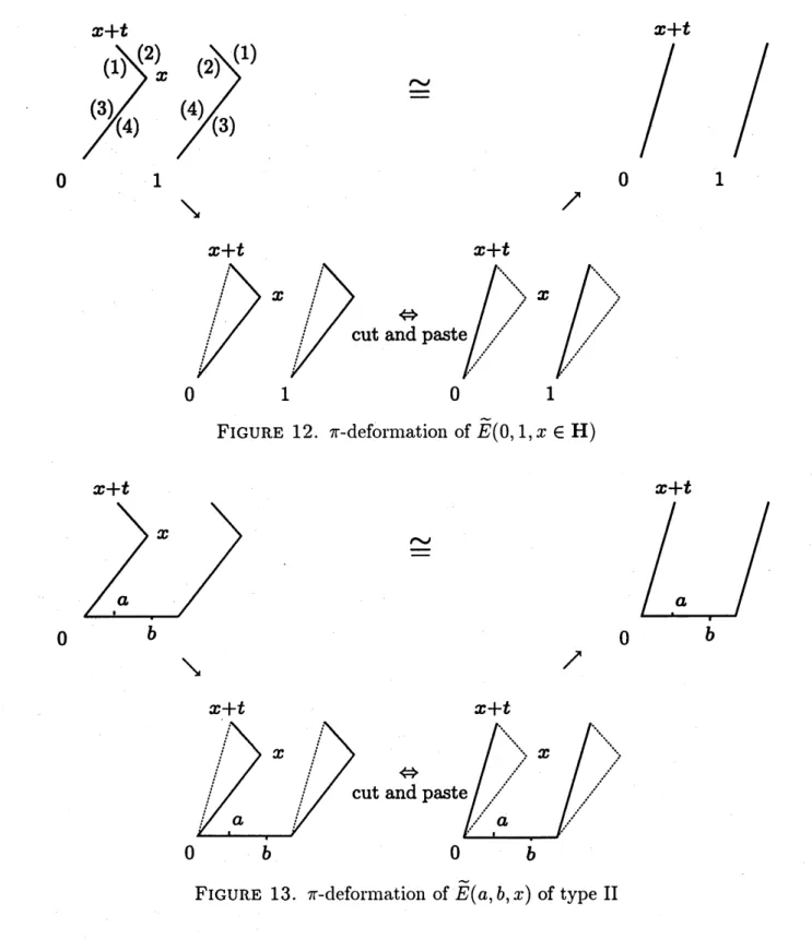
We apply a $\pi- \mathrm{d}\mathrm{e}\mathrm{f}\mathrm{o}\mathrm{r}\mathrm{n}\mathrm{l}\mathrm{a}\mathrm{t}\mathrm{i}_{0}\mathrm{n}$ to each $\overline{E}(a, b, x)$ of type I, II

or

III.

Let $p_{1}$ be the point on $\overline{E}(0,1, x)(x\in \mathrm{H})$ coming from $x$ and $x+1$, and fix

a

local

coordinate $z$

:

$\mathcal{U}_{p_{1}}arrow \mathbb{C}$ around $p_{1}$ such that $\zeta=z^{2}+x$ or $\zeta=z^{2}+x+1$, where $\zeta$

is the global coordinate of $\mathbb{C}$ as before. When we consider the coordinate

$(\mathcal{U}_{p_{1}}, Z)$, the

$\underline{\simeq}$

$0$ 1 $0$

1

$\backslash$

$\nearrow$

FIGURE 12. $\pi$-defornlation of$\tilde{E}(0,1, x\in \mathrm{H})$

$=\sim$

$0$

$\backslash$

$\nearrow$

FIGURE

13.

$\pi$-deformation of$\tilde{E}(a, b, x)$ of type II

$\zeta$-plane:

one

is from _$x$ to $x+t$ and the other is from $x+1$ to $x+1+t$. The fiber $F_{t}$

on

$t\in D_{\epsilon}$ is obtained from $\tilde{E}(0,1,x)$ by cutting and pasting along the two line segments; $F_{t}$

is equivalent to $\tilde{E}(0,1, x+t)$. (See Figure 12. The numbers (1),

...

,(4) indicate where

to paste.) Accordingly we can regard $x\in \mathrm{H}$ as a local coordinate when $a=0$ and $b=1$.

Applying a$\pi$-deformation to $\tilde{E}(\mathit{0},, b, x)$ of type II in the same way, we see that $x$ is also

$x+t.$. $\sim=$ $\sqrt$ $\sqrt$ $x+t$ $\sim_{=}$: $\sim_{=}$: $0$ $x$

1

$0$ $x$

1

$0$ $x$

1

$0$ $x$ 1 _$-x-t$

$\neg$ $\neg$ $\underline{\underline{\sim}}$ $\sim$ $\sim$ $=\sim$ $\sim \mathrm{C}$ $\sim \mathrm{C}$

$x+t$ $x+t$ $0$ 1

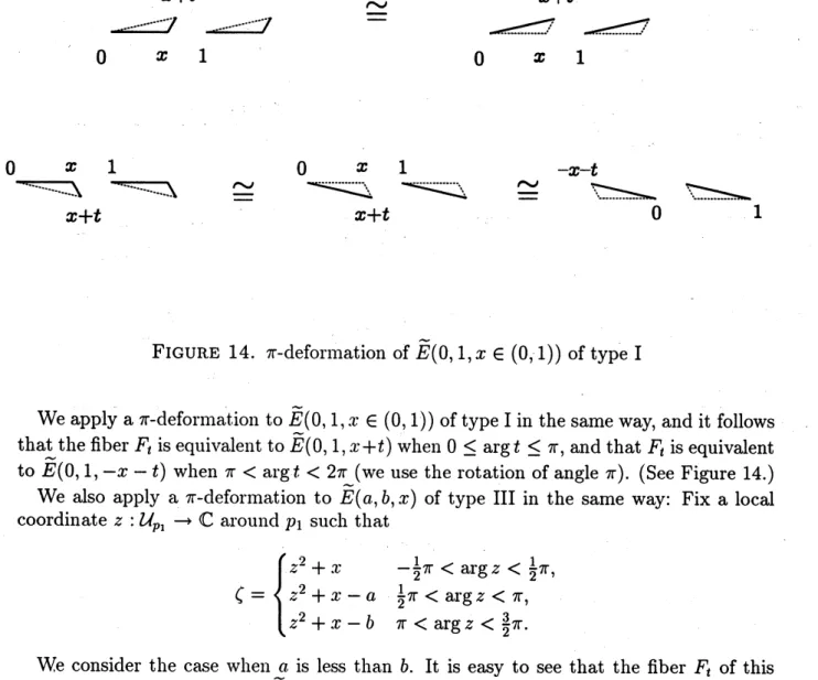
FIGURE 14. $\pi$-deformation of$\tilde{E}(0,1, x\in(\mathrm{O}, 1))$ of type I

We$\mathrm{a}\mathrm{p}\mathrm{p}\mathrm{l}\acute{\mathrm{y}}$ a$\pi-\dot{\mathrm{d}}$eformat,ion

to$\tilde{E}(0,1, x\in(\mathrm{O}, 1))$ oftype Iin the

same

way, and it follows

that the fiber $F_{t}$ isequivalent to $\tilde{E}(0,1, x+t)$ when _{$0\leq\arg t\leq\pi$}, and that $F_{t}$ is equivalent

to $\tilde{E}(0,1, -x-t)$ when _{$\pi<\arg t<2\pi$} (we use the rotation _{of angle} $\pi$). (See Figure 14.)

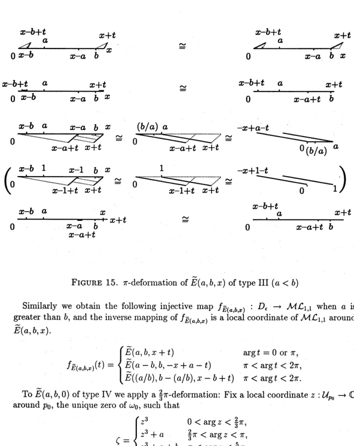
We also apply a $\pi$-deformation to $\tilde{E}(\mathit{0}, b, x)$ of type III in the same way: Fix a local

coordinate $z:\mathcal{U}_{p_{1}}arrow \mathbb{C}$ around$p_{1}$ such that

$\zeta=$

We consider the case when $a$ is less than $b$

.

It is easy to see that the fiber $F_{t}$ of this deformation is equivalent to $\tilde{E}(a, b, x+t)$ when _{$\arg t=0$}

or

$\pi$

.

When $0<\arg t<\pi$,

we

see

by

cutting

and

pasting

that $F_{t}$ is equivalent to $\tilde{E}(a, b-a, x-b+t)$

.

When

$\pi<\arg t<2\pi$ and $a\neq 1$, we see that $F_{t}$ is equivalent to $\tilde{E}(a-(b/a), (b/a),$$-X+a-t)$

where $(b/a)$ is a non-negative integer such that _{$0\leq(b/a)<a$} and $(b/a)\equiv b$ mod $a$

.

Note that $(b/a)$ is equal to $0$ if and only if _$a$ is equal to 1, and then $F_{t}$ is equivalent to

$\overline{E}(0,1, -x+1-t)$ of type I. (See Figure 15.) Accordingly

we

obtain the followinginjective

map $f_{\tilde{E}(a,b,x)}$

:

$D_{\epsilon}arrow \mathcal{M}\mathcal{L}_{1,1}$ when $a$ is less than $b$, and the inverse mapping of

$f_{\tilde{E}(a,b,x)}$ is

a local coordinate of$\mathcal{M}\mathcal{L}_{1,1}$ around $\tilde{E}(a, b, x)$.

$\cong$ $x-b+t$

a

$x+t$ $x-b+t$

a

$x+t$ $\cong$ $0\overline{x-bx}$$X$ $0\overline{x-a+tb}$ $x-b+t$ $\mathrm{o}^{\ovalbox{\tt\small REJECT}}x-b$

a

$x-a$ $bxx+t$ $\cong$ $0^{\frac{ax}{x-a+tb}}+t$ $x-a+t$

FIGURE

15.

$\pi- \mathrm{d}\mathrm{e}\mathrm{f}_{0}\mathrm{r}\mathrm{n}\mathrm{u}\mathrm{a}\mathrm{t}\mathrm{i}_{\mathrm{o}\mathrm{n}}$ of$\tilde{E}(a, b, x)$ of type III $(a<b)$

Similarly

we

obtain the following injective map $f_{\tilde{E}(b,)}a,x$

:

$D_{\epsilon}arrow \mathcal{M}\mathcal{L}_{1,1}$ when $a$ is

greater than $b$, and the inverse$\mathrm{n}\mathrm{l}\mathrm{a}\mathrm{p}\mathrm{P}^{\mathrm{i}}\mathrm{n}\mathrm{g}$ of_{$f_{\tilde{E}(a,b,x)}$} is alocal coordinate of$\mathcal{M}\mathcal{L}_{1,1}$ around

$\tilde{E}(a, b, x)$

.

$f_{\tilde{E}(a,b,x)}(t)=$

$\pi<\arg\arg t\pi<\arg t<2\pi=0\mathrm{o}\mathrm{r}t<2\pi\pi,.$

’

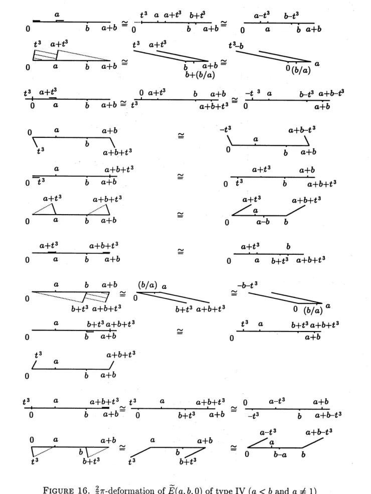
To $\tilde{E}(a, b, \mathrm{o})$ oftype IV

we

apply $\mathrm{a}\frac{2}{3}\pi$-deformation: Fix a local coordinate $z$ :$\mathcal{U}_{p_{0}}arrow \mathbb{C}$ around $p_{0}$, the unique zero of$\omega_{0}$, such that

$\zeta=$

Then the segment $s_{t}’$ is $\mathrm{t}\mathrm{l}\cdot \mathrm{a}\mathrm{n}\mathrm{S}\mathrm{f}\mathrm{e}\mathrm{r}\mathrm{r}\mathrm{e}\mathrm{d}$ to two parallel line segments with the same length $t^{3}$

in $\zeta$-plane.

$\mathrm{o}^{\frac{a}{ba+}}b\cong 0\ldots.\overline{ba+}b^{\cong}$

$a-t^{3}$ $b-t^{3}$

$t^{3}$ a $a+t^{3}$ $b+\theta$

$0\overline{aba+}b$

$\frac{t^{3}.a\underline{+t^{3}}}{\dot{0}a\dot{b}a+}b\cong t^{3}0a+t^{3}$_{$\ovalbox{\tt\small REJECT}$$baa+b+t+b3$} $-t3$ a _{$b-t^{3}a+ba+b-t^{3}$} $\cong \mathrm{o}^{\ovalbox{\tt\small REJECT}}$

$\cong$

$0\overline{\overline{t}^{3}}$

a

$b$

$a+ba+b+t^{3}$ $\cong$ $0^{\frac{a+t^{3}a+b}{t^{3}ba}}+b+t^{3}$

$\cong$

$\mathrm{o}^{\frac{a+t^{3}a+b+}{aba}}+bt^{3}$ $\cong$

$0\underline{a+t^{3}b}$

a $b+t^{3}$ $a+b+t^{3}$

$\mathrm{o}^{\frac{a}{ba+b}}$ $\cong$ $0\underline{t^{\theta}}$

a $a+b$ $b+t3a+b+t\theta$ $b+t^{s_{a+bt}3}+$ $t_{\frac{3}{0}}$a $ba+b^{\cong}a+b+t^{3}t_{\frac{3a}{0}}$ . $- a+b+t^{3} \cong\frac{0a-t^{3}a+b}{-t^{3}ba+b}-t^{3}$ $b+t^{3}$ $a+b$ $\cong$

$f_{\tilde{E}(a,b,0)}(t)=|^{\tilde{E}(}\tilde{E}(a+b^{-},b,a+b+t^{3})E(a,b,a_{b/)}+bt^{3})\tilde{E}(a,b-O,a+t^{3})\tilde{\tilde{E}\frac{E}{E}}(a,b,t^{3})(a,a+b,a+b(_{\mathit{0},,b},\mathit{0}+b^{-}+t3)a-(a,(b/a-t^{3})),t3-b)$ $\mathrm{a}\mathrm{r}\arg 0<\arg t<,\frac{1}{3}\mathrm{a}\mathrm{r}\arg t=\frac{1}{3}\pi\frac{2}{3}\pi<\arg t\mathrm{g}\mathrm{g}t=\pi<\mathrm{a}t=\frac{2}{3}\pi t=\frac{1}{3}\pi \mathrm{r}\mathrm{g}t’<\frac{2}{3}\pi \mathrm{o},,<\pi\pi’,$,

$\overline{E}(a-\sim(b/a), (b/a),$ $-t^{3}-b)$ $\pi<\mathrm{a}\mathrm{r}\mathrm{g}.t<\frac{4}{3}\pi$,

$\overline{E}(a, a+b, a+b+t^{3})$ $\arg t=\frac{4}{3}\pi$,

$\tilde{E}(a, b, t^{3})$ $\frac{4}{3}\pi<\arg t<\frac{5}{3}\pi$,

$\tilde{E}(a+b, b, a+b-t^{3})$ $\arg t=\frac{5}{3}\pi$,

$\tilde{E}(a, b-a, a-t3)$ $\frac{5}{3}\pi<\arg t<2\pi$

.

When $a=1$ and $a<b$,

$f_{\tilde{E}(1,b,0)}(t)=1^{E}\tilde{E}(1,b-1’,1)\tilde{E}(1+b,b^{-}1+b+t3)\tilde{E}(1,1+b,1+bt^{3})\tilde{E}(1,b,1+b+t3)\tilde{E}(0,1,t3^{+}b^{-t}\tilde{E}(1,b,-t^{3}(1,b,1b3))+t^{3^{-}})$ $0< \mathrm{a}\mathrm{r}\mathrm{g}\mathrm{a}\mathrm{r}\mathrm{g}\mathrm{a}\mathrm{r}\mathrm{a}\mathrm{r}\mathrm{g}\mathrm{a}\mathrm{r}\frac{1}{3}\pi<\arg t\frac{2}{3}\pi<\mathrm{a}\mathrm{r}t<\frac{1}{3}\pi \mathrm{g}t=0\mathrm{g}t=\frac{1}{3}\pi \mathrm{g}t’<\pi t=\frac{2}{3}t=\pi’,\frac{2}{3}<’,\pi\pi,$

’

$E(\mathrm{O}, 1, -t^{3}-b)$ $\pi<\arg t<\frac{4}{3}\pi$,

$E(1,1+b, 1+b+t^{3})$ $\arg t=\frac{4}{3}\pi$, $\tilde{E}(1, b, t^{3})$ $\frac{4}{3}\pi<\arg t<\frac{5}{3}\pi$,

$\tilde{E}(1+b, b, 1+b-t^{3})$ $\arg t=\frac{5}{3}\pi$,

When $a=b=1$,

$f_{\tilde{E}(1,1,0)}(t)=$ $0.< \mathrm{a}\mathrm{a}\mathrm{r}\mathrm{g}\mathrm{a}\mathrm{r}\arg\pi_{1}\arg t=\pi \mathrm{a}\frac{1}{3}\mathrm{a}\frac{2}{3}\pi\frac{4}{3}\frac{5}{3}\mathrm{r}\mathrm{g}t=\frac{5}{3}\pi\pi<\arg t,<\frac{2}{3},\pi\pi\pi<\mathrm{a}\mathrm{r}\mathrm{g}’ t’<\mathrm{r}\mathrm{g}t=\mathrm{g}t=\frac{4}{3}\pi<\arg t<\mathrm{a}\mathrm{r}t<t==0,\frac{5}{3},\pi\arg t’<2\pi \mathrm{g}t<\frac{1}{3}\pi\pi\frac{\mathrm{l}}{3}\pi\frac{2}{3}\mathrm{g}t’<\pi<\frac{4}{3}\pi,.’$

,

When $b=1$ and $a>b$,

$f_{\tilde{E}(a,b,0)}(t)=$

For each$\overline{E}(a, b, 0)$oftype IV, the

lnap $f\tilde{E}(a,b,0)$ gives risetoa two-fold branched covering;

$f_{\tilde{E}()}a,b,0(t)=f\tilde{E}(a,b,0)(-t)$.

Then $(f_{\tilde{E}(a,b,0)}, D\mathbb{Z}/\epsilon’)2\mathbb{Z}$ gives rise to a local manifold cover of$\mathcal{M}L_{1,1}$ around $\overline{E}(a, b, \mathrm{o})$.

In this way, the set $\mathcal{M}\mathcal{L}_{1,1}$ is regarded as a complex V-manifold.

REFERENCES

[H-O1] Hashimoto, Y. and Ohba, IC.: Cutting and pasting_ofRiemann_surfaceswithAbelian differentials,

I, preprint.

[H-O2] Hashimoto, Y. and Ohba, $\mathrm{I}\zeta.$: Construction

ofRiemann _surfaces by parallel transformations, to

appear in 数理解析研究所講究録

[K] Kodaira, $\mathrm{I}\backslash ^{r}.$: Complex

Manifolcls and _{Deformation of} Complex Structures, Grund. Math. Wiss.

283, Springer-Verlag, New$\mathrm{Y}^{r}\mathrm{o}\mathrm{r}\mathrm{k}-\mathrm{B}\mathrm{e}\mathrm{r}\mathrm{l}\mathrm{i}\mathrm{n}$-Heidelberg-Tokyo, (1986).

[Mo] Morelli, R.: A theory _ofpolyhedra, Adv. in Math. 97 (1993), 1-73.

[Mu] Mumford, D.: Tata Lectures on Theta I, Progress in Mathematics vol. 28, Birkh\"auser,

Boston-Basel-Stuttgart, (1983).

[S] Sah, C-H:Hilbert’s th.irdproblem: scissors congruence, Research Notes in Mathematics 33, Pitman

Advanced Publishing Program, San $\mathrm{F}_{\Gamma \mathrm{a}\mathrm{n}\mathrm{C}}\mathrm{i}\mathrm{s}\mathrm{c}0^{-}\mathrm{L}\mathrm{o}\mathrm{n}\mathrm{d}_{0\mathrm{n}\mathrm{M}\mathrm{e}\mathrm{l}\mathrm{b}\mathrm{o}\mathrm{u}\mathrm{r}}-\mathrm{n}\mathrm{e}$ , (1979).

(Yoshitake HASHIMOTO) DEPARTMENT OF MATHEMATICS, FACULTY OF SCIENCE, OSAKA CITY

UNIVERSITY, SUGIMOTO, $\mathrm{S}\mathrm{U}\mathrm{M}\mathrm{I}\mathrm{Y}\mathrm{o}\mathrm{s}\mathrm{H}1- 1\backslash \prime \mathrm{U}$, OSAKA 558, JAPAN

$E$-mail address: $\mathrm{h}\mathrm{a}\mathrm{s}\mathrm{h}\mathrm{i}\mathrm{m}\mathrm{o}\mathrm{t}\emptyset \mathrm{s}\mathrm{C}\mathrm{i}$.osaka-cu.ac.jp

(Kiyoshi OHBA) DEPARTMENT OF MATHEMATICS, FACULTY OF SCIENCE, OCHANOMIZU

UNIVER-SITY, OTSUKA 2-1-1, $\mathrm{B}\mathrm{U}\mathrm{N}\mathrm{I}\{\mathrm{Y}\mathrm{O}- \mathrm{I}\backslash \mathrm{U}r,$ $\mathrm{T}\mathrm{o}\mathrm{I}\backslash \mathrm{Y}\mathrm{o}112$, JAPAN