JAIST Repository: System-Level Performance Evaluations of Spatio-Temporal Equalizers Using Two-Dimensional Channel Sounding Field Measurement Data

Japan Advanced Institute of Science and Technology

JAIST Repository

https://dspace.jaist.ac.jp/

Title

System-Level Performance Evaluations of

Spatio-Temporal Equalizers Using Two-Dimensional Channel

Sounding Field Measurement Data

Author(s)

Matsumoto, Tad; Yamada, Takefumi; Tomisato,

Shigeru

Citation

Proceedings of the XXVIIth General Assembly of

International Union of Radio Science (URSI GA

2002)

Issue Date

2002-08

Type

Conference Paper

Text version

publisher

URL

http://hdl.handle.net/10119/9125

Rights

Copyright (C) 2002 URSI. Tad Matsumoto, Takefumi

Yamada, and Shigeru Tomisato, Proceedings of the

XXVIIth General Assembly of International Union

of Radio Science (URSI GA 2002), 2002.

System-Level Performance Evaluations of Spatio-Temporal Equalizers Using Two -Dimensional

Channel Sounding Field Measurement Data

Tad Matsumoto, Takefumi Yamada, and Shigeru Tomisato NTT DoCoMo, Inc.

3-5 Hikari-no-oka, Yokosuka-shi, Kanagawa-ken 239-8536, Japan TEL: +81-468-40-3227, FAX: +81-468-40-3790

E-mail: {matumoto, fumi, tomisato}@mlab.yrp.nttdocomo.co.jp

1. INTRODUCTION Recently, joint spatio-temporal equalization (S/T-Equalization) techniques have been recognized as potential technological basis that can achieve significant enhancement in signal transmission performances over broadband mobile communication channels. S/T-Equalization is a unified concept combining adaptive array antennas and temporal equalizer concepts. Obviously, a purpose of S/T-Equalization is to endow receivers with the immunity against co-channel interference (CCI) and inter-symbol interference (ISI), aiming at allowing all users to use the same frequency- and time-slots without spreading their signals in the frequency domain.

Various signal processing algorithms for S/T-equalizers have been proposed. Refs. [1] and [2] survey the historical background of the technology, and summarize current trends in S/T-equalizer algorithm development. Despite the volume of efforts made on algorithm development, few papers have examined in-field performance [3]-[5]. We have presented initial investigation results on the effectiveness of S/T-Equalization techniques under real mobile radio propagation environments through link-level simulations using two-dimensional channel sounding field measurement data [6], [7]. The link-level simulation focuses on analyzing/evaluating the impact of S/T-equalizer configurations, parameters, and algorithms on performance in the field. A reasonable extension of the link-level simulations is the simulations that aim to obtain system-level performance figures such as geographical distribution of signal-to-interference plus noise power ratio (SINR) in the areas of interest as well as outage probability.

The main focus of this paper is to evaluate outage probabilities of a cellular communication system featuring an S/T-equalizer, taking into account the presence of multiple interferers that use the same time- and frequency-slots. Two-dimensional channel sounding field measurement data gathered in a typical urbane area of Tokyo is used in the simulations. This paper is organized as follows: Section 2 describes in detail the S/T-equalizer configuration investigated in this paper. The algorithm used to determine the tap weights in the S/T-equalizer is also presented in Section 2. In Section 3, the simulation methodology for evaluating system-level performance figures of the S/T-equalizer using two-dimensional channel sounding field measurement data is introduced. In section 4, uplink outage probabilities for various S/T-equalizer configurations, obtained as results of the simulations, are presented. Finally, a major conclusion of this paper is drawn in Section 5.

2. S/T-EQUALIZER CONFIGURATION Configurations of the S/T-equalizer investigated in this paper, and the

algorithm for determining the S/T-equalizer tap weights are described in this section. Figure 1 shows a block diagram of the S/T-equalizer. It consists of a cascaded connection of adaptive array antenna and the maximum likelihood sequence estimator (MLSE) [6], [7]: each of the adaptive array antenna elements is equipped with a fractionally spaced tapped delay line (FTDL), and MLSE has taps covering a portion of the channel delay profile (This S/T-equalizer configuration is referred to as FTDL/MLSE for convenience). MLSE estimates the sequence considered most likely to have been transmitted.

Key parameters are the numbers L, M, and N of the antenna elements, the FTDL taps, and the taps in MLSE, respectively, which are expressed as (L, M, N) for notation convenience. The N taps in MLSE are used to replicate the signal at the array output corresponding to the symbol sequence selected by MLSE. There are LM+N taps that have to be adaptively determined according to the channel conditions such as incident angles and strengths of the desired and interference users’ multipath components. MLSE uses the Viterbi algorithm, for which the number of the states is Q(N-1) for Q-level signaling. For quaternary phase shifted keying (QPSK), Q=4.

The LM+N tap weights are determined so that

min,

→

X

W

H

(1)

where vectors Wand X are the weight and sampled data vectors, respectively. The first LM entries of W are the tap weights on the L antenna elements, and the following N entries are the MLSE taps, as

W

=

[

W

_a

,

W

_t

]

T with

]

[

_{a11 a12 a1M a21 a22 a2M aL1 aL2 aLM} a

=

W

,

W

,

L

,

W

,

W

,

W

,

L

,

W

,

L

,

W

,

W

,

L

,

W

W

(2) and

]

[

_{t1 t2 tN} t

=

W

,

W

,

L

,

W

W

. (3)

The data vector X has the same structure as W, as

X

=

[

X

_a

,

X

_t

]

Twith

]

[

_{a11 a12 a1M a21 a22 a2M aL1 aL2 aLM} a

=

X

,

X

L

,

X

,

X

,

X

L

,

X

,

L

,

X

,X

L

,

X

X

(4) and

]

[

_{t1 t2 tN} t

=

X

,

X

,

L

,

X

X

. (5)

Elements of Xa are of the samples taken at the outputs of FTDL on the L antenna elements. During the training period,

elements of Xt are the sequence of signal points corresponding to the signal reference (= unique word sequence)

transmitted at the head of the frame.

A constraint on the first MLSE tap wt1 being -C (=Constant) has to be imposed in order to eliminate the trivial

solution where all the weights are determined to be zero (It is obvious that without this constraint, a solution to Eq. (1)’s optimization problem is

W

a

=

0

and

W

t

=

0

). With this constraint, Eq. (1) is equivalent to

min,

CX

'

'

X

−

_t1

→

W

H (6)

where

W

'

=

[

W

_a

,

W

'

_t

]

Tand

X'

=

[

X

_a

,

X

'

_t

]

Twith

W

'

_t

=

[

W

_t2

,

L

,

W

_tN

]

and

X

'

_t

=

[

X

_t2

,

L

,

X

_tN

]

.

Since Eq. (6) is a standard minimum mean square estimation (MMSE) problem, the tap weights can be determined recursively by using the recursive least square (RLS) algorithm.

3. SIMULATIONS

3.1 FIELD MEASUREMENTS The primary purpose of the simulations is to evaluate system-level performance attributes such as outage probability of a system using the S/T-equalizer, for which geographical distributions of parameters in a certain area of interest have to be calculated. For this purpose, many sets of impulse response data have to be gathered at many points in the area of interest. A series of two -dimensional channel sounding measurements was conducted in Ikebukuro, a typical urban area in Tokyo.

A two-dimensional channel sounder was used in the field measurement. The carrier frequency of the channel sounding signal was 5.2 GHz. The receiver antenna of the channel sounder was located on top of a building whose height was 32 meters. Other surrounding buildings had almost the same height. An eight-element uniform linear array (ULA) was used as the sounder’s receiver antenna. Figure 2 shows a map of the measurement area. BSA indicates the

position of the desired user’s home base station where the channel sounder’s eight-element ULA was located. Channel sounding signal was transmitted from the points belonging a big triangle comprised of the Sectors A1, B1, B2, and B3 at

different times, and 41 sets of CIR data were collected. Output of the field measurement was sets of data indicating the measured impulse responses of the channels between the transmitter’s omni-directional antenna and each of the ULA ’s eight elements.

3.2 SIMULATION METHODOLOGY Four users were considered in the simulations. They were located in the sectors A1, B1, B2, and B3’s combined triangle. The users were assumed to communicate with one of their surrounded

base stations. The geographical cell boundaries indicated by the dashed lines in Fig . 3 do not necessarily indicate the boundaries of the base stations’ serving areas. Each user’s communicating base station was determined based on the strength of signal received by the base stations BSA, BSB, BSC, BSD, BSE, or BSF.

If a user is found to be in the sector A1, this user may communicate with BSA, BSB, BSC, or BSE. With which

base station the user communicates depends on the path-loss and shadowing. Assuming that the attenuation in signal strength due to the path-loss is proportional to the 3.7th power of distance, and that shadowing is an independent random variable distributed over a Log-Normal distribution with standard deviation of 10.0 dB, overall losses with the channels between this user and each of the base stations BSA, BSB, BSC, and BSE were calculated. The base station

having the smallest overall path loss is then chosen as this user’s home base station. Similarly, if a user is found to be in the sector B1, he may communicate with BSB, BSC, or BSD; a user in B2 with BSA, BSB, BSC, or BSE, and a user in the

sector B3 with BSB, BSE, or BSF. Which of the base stations the users communicate with is determined in the same way

as for the user in the sector A1. As easily understood, the only mechanism that produces randomness in the received

signal strength is the shadowing. It was assumed that one base station serves one user. If multiple users are determined to be served by the same base station, the losses due to shadowing with the users were re -generated.

The user who was determined to communicate with BSA was the desired user, and the rest of the four users

were interferers. Pass-losses due to the distances between each interferer’s location and BSA were also calculated, and

their corresponding shadowing losses were computer-generated, and multiplied by the pass-losses. The desired and interference users were assumed to be power-controlled by their communicating base stations so that the received signal-to-noise power ratio (SNR) becomes 15 dB. The effect of the power control on strengths of the interferers’ signals received by BSA was then taken into account.

10000 combinations were taken by randomly choosing the desired and three interference users’ locations from among the 41 field measurement points within the four sectors’ combined big triangle. For each of the 10000 combinations, the overall channel losses due to the distance, shadowing, and power-control were calculated, and the channel losses were multiplied by the field measurement CIR data. The signal processing for the S/T-equalizer was then performed, and cumulative distribution function of the MLSE input SINR defined as

Algorithm

RLS

the

of

e

Convergenc

after

Error

Squared

Mean

Energies

Path

Combinable

of

Total

SINR

=

(7)

was evaluated using the 10000 combinations of the field measurement data.

4. RESULTS

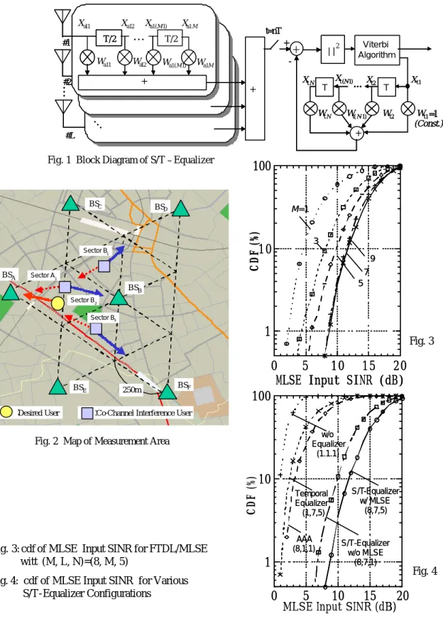
4.1 FTDL TAP NUMBER A purpose of using FTDL is to enhance MLSE input SINR and to relax performance sensitivity to symbol timing offset. Figure 3 shows cumulative distribution function of the MLSE input SINR for FTDL/MLSE with (L, M, N) = (8, M, 5) with M as a parameter. It is found that better performance can be achieved with larger FTDL length: 8.5 dB MLSE input SINR can be achieved at 99% of the service area when (L, M, N) = (8, 7, 5), but the difference between (8, 9, 5) and (8, 7, 5) is very minor. Compared with the (8, 1, 5) configuration, (8, 7, 5) can achieve approximately 6 dB performance imp rovement at 1% outage.

4.2 COMPARISON WITH SIMPLER CONFIGURATIONS Figure 4 shows cumulative distribution functions of the

MLSE input SINR for (L, M, N)=(8, 7, 5), (8, 1, 1), (1, 7, 5), and (1, 1, 1). Obviously, the performance with the (1, 1, 1) configuration is the worst among them. Systems using the (1, 1, 1) configuration (=non-adaptive omni-directional antenna) may need spreading of the signals in the frequency domain to achieve the process gain at the receiver side. Neither the (1, 7, 5) configuration (=omni-directional antenna with FTDL/MLSE temporal-equalizer) nor the (8, 1, 1) configuration (=8-element adaptive array antenna) achieves reasonable performance if the requirement for the system outage is 1%. Even if the outage requirement is 10%, they need auxiliary technique such as error correcting coding that has to work properly with 2...3 dB SINR.

The (8, 7, 1) configuration (S/T-equalizer without MLSE) achieves much better performance than the (1, 1, 1), (1, 7, 5), and (8, 1, 1) configurations: if the requirement for the system outage is 1%, the receiver has to work properly with 7 dB input SINR. Obviously, the (8, 7, 5) configuration achieves the best performance: the cumulative distribution curve for (8, 7, 5) indicates that at 99% of the sector A1, the MLSE input SINR can be made larger than or equal to 8.5 dB. In

fact, 8.5 dB input SINR is sufficient for MLSE to achieve acceptable level of BER, say, 10-6, that would support multi-media communications, with a help of simple error correction coding.

5. CONCLUSIONS The main focus of this paper has been on evaluating outage probabilities of cellular communication systems featuring an S/T-equalizer. Assuming a sectored cell layout, cumulative distribution function of the MLSE input SINR was evaluated, taking into account the presence of multiple interferers that use the same time- and frequency-slots. Two-dimensional channel sounding filed measurement data collected in a downtown area of Tokyo was run to perform algorithm for the S/T-equalizer in the simulations. The S/T-equalizer investigated in this paper has an (L, M, N) configuration where each of the L antenna elements is equipped with a fractionally spaced tapped delay line (FTDL) having M taps, and the temporal equalizer has N taps covering a portion of the channel delay profile to perform the maximum likelihood sequence estimation (MLSE). The most significant finding of this paper is that with the (8, 7, 5) S/T-equalizer configuration, MLSE’s input SINR can be made larger than or equal to 9.5 dB at 99% of the sectored area tested.

References [1] A. J. Paulraj and C.B. Papadias, “Space-Time Processing for Wireless Communications”, IEEE Signal Processing Magazine, pp. 49-83, Nov. 1997 [2] Ryuji Kohno, “Spatial and Temporal Communication Theory Using Adaptive Antenna Array”, IEEE Personal Communications, pp. 28-35, Feb. 1998 [3] R.S. Thomä, D. Hampicke, A. Richter, G. Sommerkorn, A. Schneider, U. Trautwein, and W. Wirnitzer, “Identification of Time-Variant Directional Mobile Radio Channels”, IEEE Trans. on

in Mobile Communications” IEEE ComMag, vol. 34, No.2, Feb. 1996, pp. 70-81 [5] U. Trautwein, D. Hampicke, G. Sommerkorn, and R.S. Thomä, “Performance of Space-Time Processing for ISI- and CCI Suppression in Industrial Scenarios”, Proc. IEEE VTC2000-Sprig, T okyo, Japan, May 15-18 2000. [6] T. Yamada, S. Tomisato, T. Matsumoto, and U. Trautwein, “Results of Link-Level Simulations Using Field Measurement Data for an FTDL-Spatial/ MLSE -Temporal Equalizer“, IEICE Trans. Commun., Vol. E84-B, No. 7 July 2001, pp. 1956-1960 [7] T. Yamada, S. Tomisato, T. Matsumoto, and U. Trautwein, “Performance Evaluation of FTDL-Spatial/MLSE-Temporal Equalizers in the Presence of Co -Channel Interference – Link-Level Simulation Results Using Field Measurement Data -“, IEICE Trans. Commun., Vol. E84-B, No. 7 July 2001, pp. 1961-1964

t=nT T Viterbi Algorithm ＋ T … + | |2 + - =1 (Const.)

…

…

T/2 W_a11 #1 #2 #L + +

…

T/2

W_a12 Wa1(M-1) Wa1M

X_a12

Wt N Wt( N- 1) Wt2 Wt1

X_{t N} Xt (N-1) X_t2 Xt1

X_a11 X_a1(M-1) X_a1M

t=nT T Viterbi Algorithm ＋ T T … + | |2 | |2 + - =1 (Const.)

…

…

T/2 W_a11 #1 #2 #L + + +

…

T/2 T/2

W_a12 Wa1(M-1) Wa1M

X_a12

Wt N Wt( N- 1) Wt2 Wt1

X_{t N} Xt (N-1) X_t2 Xt1

X_a11 X_a1(M-1) X_a1M

：Desired User ：Co-Channel Interference User

BSA BS_{C BS} D BSB BS_E BSF 250m Sector B₁ Sector B2 Sector B3 Sector A₁

：Desired User ：Co-Channel Interference User

BSA BS_{C BS} D BSB BS_E BSF 250m Sector B₁ Sector B2 Sector B3 Sector A₁

1

10

100

0

5

10

15

20

CDF (%)

MLSE Input SINR (dB)

M=1 3 5 7 9

1

10

100

0

5

10

15

20

CDF (%)

MLSE Input SINR (dB)

M=1 3 5 7 9

1

10

100

0

5

10

15

20

w/o Equalizer (1.1.1) S/T-Equalizer w/o MLSE (8,7,1) AAA (8,1,1) Temporal Equalizer (1,7,5) S/T-Equalizer w/ MLSE (8,7,5)

CDF (%)

MLSE Input SINR (dB)

1

10

100

0

5

10

15

20

w/o Equalizer (1.1.1) S/T-Equalizer w/o MLSE (8,7,1) AAA (8,1,1) Temporal Equalizer (1,7,5) S/T-Equalizer w/ MLSE (8,7,5)

CDF (%)

MLSE Input SINR (dB)

Fig. 1 Block Diagram of S/T – Equalizer

Fig. 2 Map of Measurement Area

Fig. 3

Fig. 4 Fig. 3: cdf of MLSE Input SINR for FTDL/MLSE

witt (M, L, N)=(8, M, 5)

Fig. 4: cdf of MLSE Input SINR for Various S/T-Equalizer Configurations