JAIST Repository: Entrainment-enhanced neural oscillator for rhythmic motion control

JAIST Repository

Title Entrainment-enhanced neural oscillator for rhythmic motion control

Author(s) Yang, Woosung; Nak Young, Chong; Kim, Chang Hwan; You, Bum Jae

Citation Intelligent Service Robotics, 1(4): 303-311 Issue Date 2008-10

Type Journal Article

Text version author

URL http://hdl.handle.net/10119/8816

Rights

This is the author-created version of Springer, Woosung Yang, Nak Young Chong, Chang Hwan Kim and Bum Jae You, Intelligent Service Robotics, 1(4), 2008, 303-311. The original publication is available at www.springerlink.com,

http://dx.doi.org/10.1007/s11370-008-0031-6 Description

Entrainment-enhanced Neural Oscillator for

Rhythmic Motion Control

We propose a new neural oscillator model to attain rhythmic movements of robotic arms that features enhanced entrainment property. It is known that neural oscillator networks could produce rhythmic commands efficiently and robustly under the changing task environment. However, when a quasi-periodic or non-periodic signal is inputted into the neural oscillator, even the most widely used Matsuoka’s neural oscillator (MNO) may not be entrained to the signal. Therefore, most existing neural oscillator models are only applicable to a particular situation, and if they are coupled to the joints of robotic arms, they may not be capable of achieving human-like rhythmic movement. In this paper, we perform simulations of rotating a crank by a two-link planar arm whose joints are coupled to the proposed entrainment-enhanced neural oscillator (EENO). Specifically, we demonstrate the excellence of EENO and compare it with that of MNO by optimizing their parameters based on simulated annealing (SA). In addition, we show an impressive capability of self-adaptation of EENO that enables the planar arm to make adaptive changes from a circular motion into an elliptical motion. To the authors’ knowledge, this study seems to be the first attempt to enable the oscillator-coupled robotic arm to track a desired trajectory interacting with the environment.

Keywords Biologically inspired Control, Neural Oscillator, Entrainment, Rhythmic Arm Motion, Crank Rotation, Simulated Annealing

1. Introduction

A network of coupled neural oscillators in the spinal cord known as Central Pattern Generators (CPGs) allows vertebrates to move in an efficient way adapting to changing terrain conditions. Specifically, most vertebrates locomote with an inherent rhythm determined by the natural frequency of their body. Particular attention should be paid to the entrainment property of neural oscillators, enabling them to lock onto the frequency of an input signal over a range of frequencies. This entrainment process plays a key role in vertebrates to adapt the nervous system to the natural frequency of the body. In our daily lives, continuous rhythmic arm movements such as turning a steering wheel, rotating a crank, etc. are self-organized through the interaction between the musculo-skeletal

of a robotic arm, it may efficiently provide alternate motor commands for the movement of the muscles. Then its entrainment property enables the arm to deal with environmental perturbations appropriately through afferent feedback of sensory signal. Thus, the neural oscillator’s entrainment property plays an important role in accomplishing the arm’s rhythmic motions under changing environmental and operational conditions.

Matsuoka proposed a neural oscillator model for generating rhythmic patterned outputs and analyzed the necessary conditions for self-sustained oscillations [1]. He also investigated the mutual inhibition network to control the frequency and pattern in his oscillator [2], but did not address the effect of entrainment.

Specifically, the neural oscillator can create complicated and adaptive outputs by incorporating sensory input from the environment. Thus, if the neural oscillator is coupled to the dynamical system, it can be effectively used as a reactive controller under unknown real-world environments. Using Matsuoka’s neural oscillator (MNO), Taga et al. considered the sensory signal feedback from the joints of a biped robot [3], [4], showing that the MNO made the robot robust to the perturbation through entrainment. This approach was applied later to different locomotion systems [5], [6], [7]. Besides the examples of locomotion, various efforts have been made to strengthen the capability of robots from biological inspired neural controllers. Williamson created a humanoid arm motion based on postural primitives [8], where the spring-like joint actuators allowed the arm to safely deal with unexpected collisions sustaining cyclic motions. He also

proposed the neuro-mechanical system that was coupled with the neural oscillator for controlling rhythmic arm motions [9].

In the above-mentioned researches, even though natural adaptive motions were accomplished by the coupling between the arm joints and neural oscillators, the correctness of the desired motion was not guaranteed. For instance, robot arms are required to trace a trajectory for certain type of tasks, thus we need to focus on the end-effector tracking accuracy. For this, a new neural oscillator model with enhanced entrainment property (EENO) was recently proposed by Yang and Chong [10], [11], [12]. In order to make the neural oscillator easily adaptable for a wide variety of the input signals like quasi-periodic or non-periodic inputs, they added a new control term to the MNO.

This paper compares and contrasts the entrainment property of a two-link planar arm implemented by the EENO and the MNO for achieving the crank rotation task. In Section II, we briefly describe the mathematical form of the EENO. In Section III, we address how to determine the optimal parameters of the EENO for a desired task. More details of the entrainment performances of both models under changing task conditions are discussed in Section IV and conclusions are drawn in Section V.

2. Entrainment-enhanced Neural Oscillator

Rhythmic motor patterns of vertebrates are obtained from the CPG and modified by sensory signals that detect environmental disturbances. Similarly, artificial neural oscillators are entrained with external stimuli at a sustained frequency. This section begins with a description of the mathematical model of the MNO and explains how it can be modified to fit the needs of enhanced entrainment, leading to the EENO as shown in Fig. 1.

Fig. 1 Schematic diagram of the EENO

The MNO is modeled by the following set of differential equations.

, 1 1 [ ] n n r ei ei fi fi i j ij j ei i i i i T x x w y w y bv k g + s = = + = − −

∑

∑

ei ei ei ei av v bI y T & + + = ) 0 , max( ] [ _{ei ei} ei x x y = + = i n i i i fi n j i ij j ei ei fi fi rx x w y w y bv k g s T + = − −

∑

∑

where xei and xfi indicate the inner state of the i-th neuron for i=1~n, which

represents the firing rate. Here, the subscripts ‘e’ and ‘f’ denote the extensor and

flexor neurons, respectively. ve(f)i represents the degree of adaptation and b is the

adaptation constant or self-inhibition effect of the i-th neuron. The output of each

neuron ye(f)i is taken as the positive part of xi and the output of the oscillator is the

difference in the output between the extensor and flexor neurons. wij is a

connecting weight from the j-th neuron to the i-th neuron: wij are 0 for i≠j and 1

for i=j. wijyi represents the total input from the neurons arranged to excite one

neuron and to inhibit the other, respectively. Those inputs are scaled by the gain

ki. Tr and Ta are the time constants of the inner state and the adaptation effect,

respectively, and si is an external input with a constant rate. we(f)i is a weight of the

extensor neuron or the flexor neuron and gi indicates a sensory input.

Since entrainment can be considered as the tracking of sensory feedback signals, it is very similar to conventional feedback controllers. Specifically, the MNO has the form of a proportional-derivative controller, if we rearrange Eq. (1) as the following 2-nd order differential equations.

i e a f f f f a e e r a e r aTx T T x x Tw y w y Tk g kg by s

T _&& +₍ + _)& + =− _& − − _[&]+− _{[ ]}+− +

(2) i f a e e e e a f f r a f r aTx T T x x Tw y wy Tkg kg by s T +₍ + ₎ + =− − − _{[ ]}−− _{[ ]}−− + & & & && (3) Now, subtracting Eq. (3) from Eq. (2) gives

), ] [ ] ([ ) ] [ ] ([ ) ( ) ( ) ( ) ( _{+ + = − + − − − −} +₋ − ₋ +₋ − +T T y y Tw y y wy y b y y Tk g g k g g y T

where Y=xe-xf . It was assumed that the inhibitory connecting weights we and wf

are identical: i.e., w ≡ we = wf. The stable oscillatory output of the neural oscillator

is obtained by inhibitory connection between the extensor and flexor neurons. Thus, if xe>0 and xf<0, or if xe<0 and xf>0, Eq. (4) can be rewritten as

, ) ( ) ( _{a r a a in in} r aTY T T Y Y TwY w bY TkG kG

T &&+ + &+ = &+ − − & − (5)

where Gin=[g]+-[g]-. In Eq. (5), the output of the neural oscillator is entrained to

the sensory feedback, Gin. Now, one can notice that this equation is similar to the

proportional-integral-derivative (PID) controller given by

, ) ( ) ( ) ( ) ( 0 2 1 2 1 ⎥ ⎦ ⎤ ⎢ ⎣ ⎡ − + − + − = + + +

_∫

where τ1 and τ2 are the time constants, respectively. R is the reference input and K

is the proportional gain. TI is the integral gain or reset time and TD is the

derivative time. A is the system constant in terms of plant parameters.

By comparing Eqs. (5) and (6), one can come to understand why we add the

integral terms, Ie and If, to the MNO as shown in Fig. 1. With the integral terms,

we finally have the EENO given by

, 1 1 [ ] n n r ei ei fi fi _{i j} ij j ei _i i i i T x x w y w y bv k g + s = = + = − −

∑

∑

∑

∑

∑

∑

3. Two-link Planar Arm coupled with Oscillators

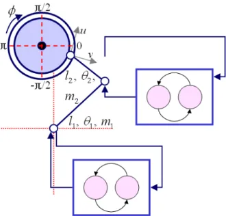
This section addresses how to couple the neural oscillator with a two-link planar arm rotating a crank. Fig. 2 illustrates a schematic model of two-link planar arm whose joints are coupled to the neural oscillator. The desired torque

command generated by the neural oscillator at the i-th joint is given by

, ) ( _{vi i i i} i i k θ θ bθ τ = − − & (8)

where ki is the position gain, bi is the velocity gain, θi is the actual angle, and θvi is

the desired angle of the i-th joint, respectively. Specifically, θvi is the output of the

neural oscillator that produces rhythmic commands of the i-th joint of the arm. The oscillator entrains the feedback signal from the joints so that the arm can exhibit adaptive motions interacting with the environment. The important thing to implement this method is how to incorporate the feedback signal’s amplitude as well as its phase, because existing oscillators usually fail to follow the feedback signal amplitude envelope.

Fig. 2 Schematic model for crank rotation task of two-link planar arm whose joints are coupled to the neural oscillator. The origins of the crank and two-link planar arm are fixed.

Now we describe the kinematics of the above-mentioned system. If the origin of

the crank center is (x0, y0), then the end-effector position of the two-link arm

denoted by (x,y) can be represented in Cartesian coordinates as

θ θ θ θ θ φ φ φ φ φ φ φ φ θ θ φ φ φ φ φ φ & & & && && & && & && && & & & & & ) , ( ) ( cos sin sin cos ) ( cos sin sin cos 2 2 12 2 1 1 12 2 1 1 0 0 J J r r r r y x J r r y x s l s l c l c l y r x r y x + = ⎟⎟ ⎠ ⎞ ⎜⎜ ⎝ ⎛ + − − − = ⎟⎟ ⎠ ⎞ ⎜⎜ ⎝ ⎛ = ⎟⎟ ⎠ ⎞ ⎜⎜ ⎝ ⎛− = ⎟⎟ ⎠ ⎞ ⎜⎜ ⎝ ⎛ ⎟⎟ ⎠ ⎞ ⎜⎜ ⎝ ⎛ + + = ⎟⎟ ⎠ ⎞ ⎜⎜ ⎝ ⎛ + + = ⎟⎟ ⎠ ⎞ ⎜⎜ ⎝ ⎛ (9) Eq. (9) can be rearranged as

), ) ( ) ( ( ) , ( )

(_{θ θ&& &θ θ&θ& φφ&& φφ&}2

v u r J J + = − (10)

where J is the Jacobian matrix of [x, y]T. φ and θi are the crank angle and the i-th

joint angle, respectively. li is the i-th link length. c1, c12, s1 and s12 denote cosθ1,

cos(θ1+ θ2), sinθ1, and sin(θ1+ θ2), respectively. r is the radius of the crank. u is

the tangential unit vector and v is the normal unit vector at the outline of the crank. These vector directions are shown in Fig. 2, respectively.

The description of dynamics of the same system is given below. The crank has the moment of inertia, I, and the viscous friction at the base joint, C. Regarding the arm dynamics, M is the inertia matrix, V is the Coriolis/centripetal vector, and G is the gravity vector. Now, the dynamic equilibrium equations of the crank and two-link arm are given in the following forms, generating a constraint and an appropriate external force.

F ru C I_{φ&&+ &φ= (φ)}T (11) F J G V M_{(θ)θ&&+ (θ,θ&)+ (θ)=τ′− (θ)}T (12)

where τi′=τi −cθ&i for i=1~2 and c denotes the joint viscosity matrix [13]. F is

the contact force interacting between the crank and the end-effctor. By solving Eqs. (11) and (12) simultaneously using Eq. (10), F is given in the following form. ))} ( ) ( ( ) , ( )) ( ( ) ( ) ( { } ) ( ) ( ) ( ) ( ) ( {_{Jθ M θ} 1_{J θ r}2_I 1_{uφ uφ} 1 _{J θ M θ} 1_{τ V θ Jθ θ θ rφ vφφ CI} 1_uφ

F₌ − T ₊ − T − − _{′− + & & &+ & &+} −

(13)

Now the robotic arm whose joints are coupled to the neural oscillator is mathematically represented by Eqs. (8), (12) and (13).

4. Optimization of Oscillator Parameters

The neural oscillator is a non-linear system, thus it is generally difficult to analyze the dynamic response of robotic arm when the oscillator is connected to it. Therefore a graphical approach known as the describing function analysis has been proposed earlier [14]. The main idea is to plot the system response in the complex plane and find the intersection points between the Nyquist plots of the robotic arm and neural oscillators. The intersection points indicate limit cycle solution. However, even if rhythmic arm motions can be generated by this method, it may not be possible to obtain the desired motion required by the task. This is because many parameters of oscillator need to be tuned appropriately, and different responses occur according to the method for managing the connection between oscillators. In this work, we propose and analyze an approach to

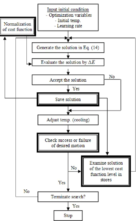
determining the optimal parameters of the oscillator based on simulated annealing [15] that enables the arm to trace the given circular path. A flowchart of the algorithm is given in Fig. 3. Simulated annealing is able to avoid local minima or maxima, but when searching for optimal parameters, it is not known whether the desired task is performed correctly with the selected parameters or not. We therefore added the task completion judgment and cost function comparison steps as represented by the bold lines in Fig. 3.

Fig. 3 Flowchart of the proposed SA for oscillator parameter optimization

The details of the algorithm are presented below. An initial state of the system is chosen at the cost function and the temperature. The state (or parameters) of the neural oscillator X is replaced by a random nearby state given by

,

1 N

X Xi= i− +ν⋅

where ν is the step size for X called learning rate and N denotes a distributed random number between [-1, 1] such as Gaussian noise. If the cost function

decreases, the new state Xi is accepted and stored. Otherwise, another state is

drawn with the transition probability, Probi(E), given by

, ) exp( ) ) ( 1 ( −Δ >γ = c E T Z (E) Probi (15)

where ∆E is the change in the cost function, and γ is a random value uniformly

distributed between 0 and 1. The temperature cooling schedule is ci=k·ci-1 (k is the

Boltzmann constant or effective annealing gain) and Z(T) is a

temperature-dependant normalization factor. If ∆E ≥0 and Probi(E) is less than γ or equal zero,

Xi is rejected.The cost function includes the kinetic energy of the crank rotation,

the energy consumed by the viscous friction of each joint, and the torque applied by the oscillator.

Fig. 4 (a) indicates a cooling state in terms of cooling schedule. Cooling or annealing gain K was set to 0.95. It can be observed in Fig. 4 (b) that the

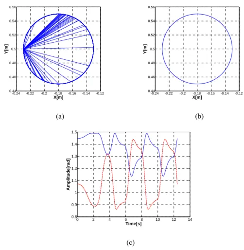
optimization process was well performed to obtain the lowest cost function. Figs. 4 (c) to (f) illustrate the procedure to determine such parameters as inhibitory connecting weight, rising and adaptation time constant, sensory gain, and tonic input gain of the EENO. We can set the converged values of these figures as the parameters of the EENO as shown in Table I. If the parameters are selected inappropriately, the given task could fail as illustrated in Fig. 5 (a). In Fig. 5 (a), the straight lines indicate the failed end-effector motions of the two-link arm. As expected, when optimal parameters are selected, a stable motion could be achieved as shown in Fig. 5 (b). It is observed from Fig. 5 (c) that there is a transient region not saturated to a stable value from 0 sec to around 4 sec., which is followed by the stable periodic motion in the next time period. As shown in Eq. (8), a PD controller is applied via torques to each joint of the two-link arm. The k and b gain of the joint 1 are 321 and 15, respectively. For the joint 2, the k gain is set to 300 and the b gain is set to 10.

Fig. 4 (a) Temperature transition for cooling schedule (b) A transition of total cost function level (c) A weight transition of inhibitory connection (d) A rising time constant transition (e) A transition of sensory gain, (f) A transition of tonic input

0 100 200 300 400 500 600 0 10 20 30 40 50 60 70 80 90 100 Number of task Te m p . 0 100 200 300 400 500 600 700 800 900 -2 0 2 4 6 8 10 Number of task T o ta l c o s t fun c tion le ve l (a) (b) 0 100 200 300 400 500 600 700 800 900 1.6 1.8 2 2.2 2.4 2.6 2.8 3 3.2 Number of task In hib itor y w e ight 0 100 200 300 400 500 600 700 800 900 0 0.5 1 1.5 2 2.5 Number of task Tr (c) (d) 0 100 200 300 400 500 600 700 800 900 0 1 2 3 4 5 6 Number of task S e nsor y gai n 0 100 200 300 400 500 600 700 800 900 58 58.5 59 59.5 60 60.5 61 61.5 62 62.5 63 Number of task To ni c i n p u t (e) (f)

Table I. Comparison between initial and optimal parameters of the EENO

Fig. 5 (a) The end-effector trajectory drawn by the two-link arm coupled with the EENO when various stable parameters are selected (b) The end-effector trajectory of the two-link arm coupled with the optimally tuned EENO (c) The output of joint angle. The red dash line is the first joint angle and the second joint angle is drawn by the blue thin line

Initial parameters Inhibitory weight (w) 2.0 Time constant (Tr) 0.25 (Ta) 0.5 Sensory gain (k) 1.0 Tonic input (s) 60.0 Optimized parameters Inhibitory weight (w) 2.5205 Time constant (Tr) 0.7651 (Ta) 1.5302 Sensory gain (k) 3.8318 Tonic input (s) 62.3519 -0.24 -0.22 -0.2 -0.18 -0.16 -0.14 -0.12 0.44 0.46 0.48 0.5 0.52 0.54 0.56 X[m] Y[m ] -0.24 -0.22 -0.2 -0.18 -0.16 -0.14 -0.12 0.44 0.46 0.48 0.5 0.52 0.54 0.56 X[m] Y[m ] (a) (b) 0 2 4 6 8 10 12 14 0.8 0.9 1 1.1 1.2 1.3 1.4 1.5 Time[s] A m pli tud e[r a d ] (c)

5. Comparison of Entrainment Property between

EENO and MNO

In this section, we compare the entrainment property between the EENO and the MNO that produces rhythmic joint commands of the two-link arm for the crank rotation task. Specifically, the circular path of the crank changes to an elliptical path instantly as shown in Case I through Case III. We assume that the x-axis and y-x-axis of Fig. 5 (b) are the diameter of the major x-axis and minor x-axis in an elliptical path, respectively. The oscillator parameters are tuned for the circular path as seen in Table II and remain unchanged for all cases. It is important to investigate whether the end-effector of the two-link arm traces the changed elliptical paths correctly or not.

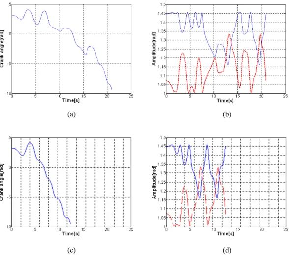
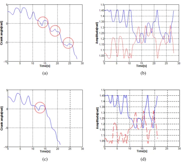
The EENO model shows better entrained movement than that of the MNO model although the path changes in the same way. Comparing Figs. 6 (a) and (b) with (c) and (d) of Case I, respectively, it can be verified that the trajectory of the crank angle in the EENO model is smoother and not fluctuant than that of the crank angle in the MNO model. Figs. 6 (a) and (c) illustrate the crank angle rotated clockwise by the two-link arm from π rad (see Fig. 2). The red dot circles of Fig. 6 (a) shows unnecessary counter-clockwise rotations of crank generated by the MNO model. The results of Case II and Case III are similar to Case I. As the path changes, the time required for entrainment increases compared with the original circular path (see Fig. 5 (c)). Particularly In Case III, even in the EENO model, the entraining time increases to 14.2 sec. Besides, if the ellipticity of the path exceeds that of Case III, both models are not moved periodically in the clockwise direction, showing that they have a limit on the range of entrainment.

From these results, it is confirmed that the neural oscillator enables a robotic arm to rhythmically move using the motor command of the extensor and flexor neurons. In addition, though a desired task changes unexpectedly, the entrainment function of the neural oscillator adjusts the control commands in an adaptive way so as to maintain rhythmic movements. It is also demonstrated that the

Table II. Comparison between optimal parameters of MNO and EENO

A. Case I: The diameter of the major axis is set to 0.5cm and that of the minor axis is set to 1cm

Optimized parameters of the MNO Inhibitory weight (w) 2.5326 Time constant (Tr) 0.6191

(Ta) 1.2382

Sensory gain (k) 2.4210 Tonic input (s) 59.2863

Optimized parameters of the EENO Inhibitory weight (w) 2.5205 Time constant (Tr) 0.7651

(Ta) 1.5302

Sensory gain (k) 3.8318 Tonic input (s) 62.3519

Fig. 6 (a) The crank angle rotated by the two-link arm coupled with MNO, (b) The joint trajectories actuated by MNO, (c) The crank angle rotated by the two-link arm coupled with EENO, (d) The joint trajectories actuated by EENO. In (b) and (d), the red dashed line is the first joint angle and the second joint angle is drawn by the blue thin line

(a) (b)

B. Case II: The diameter of the major axis is set to 1cm and that of the minor axis is set to 0.5cm

Fig. 7 (a) The crank angle rotated by the two-link arm coupled with MNO, (b) The joint trajectories actuated by MNO, (c) The crank angle rotated by the two-link arm coupled with EENO, (d) The joint trajectories actuated by EENO. In (b) and (d), the red dashed line is the first joint angle and the second joint angle is drawn by the blue thin line

(a) (b)

C. Case III: The diameter of the major axis is set to 1cm and that of the minor axis is set to 0.4cm

6. Conclusions

This paper presented the enhanced capability of entrainment of two-link planar arm coupled with the EENO to achieve a desired rhythmic motion. We

investigated how the EENO-coupled arm adjusted its joint motions to respond to an unexpected task change. Specifically, an optimization approach was proposed to determine the parameters of the EENO appropriately based on simulated annealing. Numerical examples were provided to verify the validities of the EENO and its parameter tuning method. Compared with the most widely used Fig. 8 (a) The crank angle rotated by the two-link arm coupled with MNO, (b) The joint trajectories actuated by MNO, (c) The crank angle rotated by the two-link arm coupled with EENO, (d) The joint trajectories actuated by EENO. In (b) and (d), the red dash line is the first joint angle and the second joint angle is drawn by the blue thin line

(a) (b)

was also clearly observed from the simulations that the EENO-coupled robotic arm showed self-adaptation capabilities under changing task conditions. This approach will be the first step toward the realization of biologically inspired control architecture for human-like movements. Our future work will attempt to demonstrate the validity and reliability of the proposed approach through various experiments with a real robot arm.

Acknowledgments This research was conducted as a program for the "Fostering Talent in Emergent Research Fields" in Special Coordination Funds for Promoting Science and Technology by Japan Ministry of Education, Culture, Sports, Science and Technology. This work was also supported in part by Korea MIC & IITA through IT Leading R&D Support Project.

References

1. K. Matsuoka (1985) Sustained Oscillations Generated by Mutually Inhibiting Neurons with Adaptation. Biological Cybernetics 52: 367-376

2. K. Matsuoka (1987) Mechanisms of Frequency and Pattern Control in the Neural Rhythm Generators. Biological Cybernetics 56: 345-353

3. G. Taga, Y. Yamagushi and H. Shimizu (1991) Self-organized Control of Bipedal Locomotion by Neural Oscillators in Unpredictable Environment. Biological Cybernetics 65: 147-159 4. G. Taga (1995) A Model of the Neuro-musculo-skeletal System for Human Locomotion. Biological Cybernetics 73: 97-111

5. S. Miyakoshi, G. Taga, Y. Kuniyoshi, and A. Nagakubo (1998) Three-dimensional Bipedal Stepping Motion Using Neural Oscillators-Towards Humanoid Motion in the Real World. Proc IEEE/RSJ Int Conf on Intelligent Robots and Systems pp 84-89

6. Y. Fukuoka, H. Kimura and A. H. Cohen (2003) Adaptive Dynamic Walking of a Quadruped Robot on Irregular Terrain Based on Biological Concepts. The International Journal of Robotics Research 22: 187-202

7. G. Endo, J. Nakanishi, J. Morimoto and G. Cheng (2005) Experimental Studies of a Neural Oscillator for Biped Locomotion with QRIO. Proc IEEE/RSJ Int Conf on Intelligent Robots and Systems pp 598-604

8. M. M. Williamson (1996) Postural Primitives: Interactive Behavior for a Humanoid Robot Arm. 4th _{Int. Conf. on Simulation of Adaptive Behavior. MIT Press pp 124-131}

9. M. M. Williamson (1998) Rhythmic Robot Arm Control Using Oscillators. Proc IEEE/RSJ Int Conf on Intelligent Robots and Systems pp 77-83

10. W. Yang and N. Y. Chong (2005) Dynamic Systems Control Using Entrainment-enhanced Neural Oscillator. Proc Int Conf on Control, Automation, and Systems pp 1020-1024 11. W. Yang, N. Y. Chong and B. J. You (2006) Entrainment-enhanced Neural Oscillator for Imitation Learning. Proc IEEE Int Conf on Information Acquisition pp 218-223

12. W. Yang, N. Y. Chong, C. Kim and B. J. You (2007) Optimizing Neural Oscillators for Rhythmic Movement Control. Proc IEEE Int Symp on Robot and Human Interactive Communication pp 807-814

13. H. Gomi, T. and R. Osu (1998) Task-dependent viscoelasticity of human multijoint arm and its spatial characteristics for interaction with environment. Journal of Neuroscience 18: 8965-8978 14. Jean-Jacques E. Slotine, Weiping Li (1991) Applied Nonlinear Control, Englewood Cliffs, N. J., Prentice Hall.

15. S. Kirkpatrick, C. D. Gelatt and M. P. Vecchi (1983) Optimization by Simulated Annealing. Science 220: 671-680