RELATIVE PROJECTIVITY OF CARLSON MODULES (Cohomology of Finite Groups and Related Topics)

RELATIVE

PROJECTIVITY

OF

CARLSON

MODULES

佐々木洋城 (HIROKI SASAKI)

Department

_of

Mathematical Sciences

Faculty

_of

Science, Ehime University

Matsuyama, 790-8577, JAPAN

1. INTRODUCTION

The simple

groups

of 2-rank two

were

classified about 1970 by Alperin, Brauer,

Gorenstein, Walter, and Lyons. See for example $\mathrm{A}\mathrm{l}\mathrm{p}\mathrm{e}\mathrm{r}\mathrm{i}\mathrm{n}- \mathrm{B}\mathrm{r}\mathrm{a}\mathrm{u}\mathrm{e}\mathrm{r}- \mathrm{G}_{\mathrm{o}\mathrm{r}\mathrm{e}\mathrm{n}}\mathrm{s}\mathrm{t}\mathrm{e}\mathrm{i}\mathrm{n}[3]$

.

The

2-groups ofrank two which can be Sylow 2-subgroups offinite simple

groups are

(1) dihedral 2-groups (including four-groups);

(2) semidihedral

_2-groups;.

$\cdot$

(3) wreathed 2-groups;

(4) special 2-group which is

a

Sylow 2-subgroup of $SU(3,4)$

.

All finite

groups

with these Sylow 2-subgroups above

were

determined in those works.

The cohomology algebras of finite simple

groups

of 2-rank two have been known,

dependingonthe classification theorems and

on

thefact that the cohomology algebras

of some classical

groups

were calculated. A nice oyerview of these results is in the

work by Adem-Milgram [1].

TABLE 1. Finite simple

groups

of 2-rank 2 and cohomology algebras

Remark 1.1. In Table 1 the subscript ofacohomology class indicates the degree. For

example $\rho_{4}$ is ofdegree 4, $\sigma_{6}$ is of degree 6, and so on.

From the late $1980’ \mathrm{s}$ the mod 2 cohomology algebras of those finite

groups

with

(1) dihedral and quaternion

case

by Martino-Priddy [21], 1991; by

Asai-Sasaki

[5],

1993; .

(2) semidihedral

case

by Martino [20], 1988; by Sasaki [24], 1994.

The works by Martino and Priddy dealt with the classifying

spaces,

and,

as

a

consequence, obtained the cohomology algebras. On the other hand, the works by

Asai and Sasaki depend

on

the theory of cohomology varieties of modules and

on

the modular representation theory of finite groups. Especially the theory of relative

projectivity of modules played a crucial role. The theory of projectivity of modules

relative to subgroups is fundamental in the theory of modular representations of fi-nite groups. In [17] R. Kn\"orr introduced the notion of projective

covers

of modules

relative to subgroups. In the works [4] and [5]

an

injective hull ofthe trivial module

relative to subgroups

gave

almost all information ofthe cohomology algebras. In [23]

T. Okuyama introduced the notion ofprojectivity of nodules relative to “modules”.

In the work [24]

an

injective hull of the trivial module relative to modules

was

es-sentially important. (Carlson pointed out in his lecture note [11] that the definition

of projectivity relative to modules is just

a

special

case

of the relative

_{homolog..ical}

algebra that

can

be

defined,for

a

projective class ofepimorphism.)

The purpose of this report is to show that

our

method

can

be applied to finite groups whose Sylow subgroups are

(1) extraspecial$p$

-groups

of order $p^{3}$ and of exponent $p$;

(2) wreathed 2-groups.

This work

was

done with Professor Tetsuro Okuyama.

For $H$

a

subgroup of

a

finite

group

$G$ and

an

element $\zeta$ in $H^{*}(G, k)$

we

shall often

write $\zeta_{H}$

or

$\zeta_{|H}$

,for the restriction

$\mathrm{r}\mathrm{e}\mathrm{s}_{H}\zeta$

.

2. RELATIVE PROJECTIVITY OF MODULES

2.1. Projectivity relative to subgroups. First

we

state

some

results concerning

projectivity of Carlson modules relative to subgroups. The following lemma is easy

to prove and well known. This can be used to show divisibility by a homogeneous

element.

Lemma 2.1. Let

$E_{\rho}$ : $0arrow karrow\Omega^{-1}(L_{\rho})arrow^{f}\Omega^{r-1}(k)arrow 0$

$be$ th$e$extension corresponding to

an

$el$ement$\rho$ in $H^{r}(G, k)$

.

Supposethat th$e$ Carlson

module$L_{\rho}$ is$rel$

a

tively$\mathcal{H}$-projective, where$H$ is

a

set ofsubgroupsofG. If

an

$el$ement $\xi$ in $H^{n+r}(G, k)$

sa

tisfies

$\mathrm{r}\mathrm{e}\mathrm{s}_{H}f^{*}(\xi)=0$ for every $H$ in $7i$,

where $f^{*}:$ $\mathrm{E}\mathrm{x}\mathrm{t}^{n+}(kc^{r})k,$$karrow \mathrm{E}\mathrm{x}\mathrm{t}_{kG}^{n}(L_{\rho}, k)$, th

en

there exis$ts$

an

element $\eta$ in $H^{n}(G, k)$

such that

$\xi=\rho\eta$.

The Green correspondence is

one

ofthe important tools for analyzing

indecompos-able modules. The theorem below is of fundamental importance in investigation of

Theorem 2.2. Let $\rho$ in $H^{n}(G, k)$ be ahomogen

eous

elemen

$\mathrm{t}$

.

Let $U$ be

an

indecom-posable direct summand ofthe Carlson module $L_{\rho}$ of$\rho$ with vertex D. Let $H$ be

a

$s\mathrm{u}$bgroup of$G$ containing the normalizer $N_{G}(D)$ and le

$\mathrm{t}V$ be

a

Green correspondent

of$U$ with respect to $(G, D, H)$

.

Then the Green correspondent$V$ is

a

direct summand

ofthe Carlson module$L_{(\rho_{H})}$ ofthe restriction $\rho_{H}=\mathrm{r}\mathrm{e}\mathrm{s}_{H}\rho$ to thesubgroup $H$;

more-over

the multiplici$\mathrm{t}y$ ofthe direct summand $U$ in $L_{\rho}$ is the

same

as

the $\mathrm{m}\mathrm{u}lt\mathrm{i}plicit_{\mathrm{J}’}$

of$V$ in $L_{(\rho_{H})}$

.

2.2. Projectivity relative to modules. In the rest of this section we deal with

the theory of projectivity relative to modules. See Okuyama [23]

or

Carlson [11] for

details.

Definition 2.1. For $V$

a

$kG$-module let

$P(V)=$

{

$X|X$ is

a

direct summand of $V\otimes A$ for

some

$kG$-module $A$

}.

A module in $\mathcal{P}(V)$ is said to be $P(V)$-projective

or

projective relative to $\mathcal{P}(V)$. It is

also said to be $V$-projective

or

projective relative to $V$ for short. A module is said to

be $P(V)$-injective, $in.j$

.ective relative to

$P(V),$ $V$-injective

or

injective relative to $V$ if

it is $P(V)$-projective.

Definition 2.2. An exact sequence $E:0arrow A-^{f}B-^{\mathit{9}}Carrow \mathrm{O}$ _{of $kG$-modules}

is said to be $P(V)$-split (or $V$-split for short) if $V \otimes E:0arrow V\otimes Aarrow^{f}V1\otimes\otimes B\frac{1\otimes q}{}$,

$V\otimes Carrow \mathrm{O}$ splits.

Definition 2.3. Let $M$ be

a

$kG$-module. A short exact sequence $E$ : $\mathrm{O}arrow Xarrow$

$Rarrow Marrow \mathrm{O}$ is called

a

$\mathcal{P}(V)$-projective

cover

of$M$ if

(1) $R$ is _$P(V)$-projective;

(2) $E$ is $\prime \mathrm{p}(V)$-split;

(3) the kernel $X$ has no $\mathcal{P}(V)$-projective direct summand.

If the exact sequence $E$ above is

a

$P(V)$-projective

cover

of$M$, then the kernel $X$ is

denoted by $\Omega_{P(V)}(M)$. A $P(V)$-projective

cover

is also called

a

$V$-projective

cover

and the kernel is also denoted by $\Omega_{V}(M)$. Similarly the notion of a $P(V)$-injective

hullis defined. If$F:\mathrm{O}arrow Marrow Sarrow \mathrm{Y}arrow \mathrm{O}$ is

a

$\prime \mathrm{p}(V)$-injective hull of$M$, then

the cokernel $Y$ is denoted by $\Omega_{P(V}^{-1}()M)$.

Theorem 2.3. Every $kG$-module $h$as

a

$P(V)$-projective cover, which is uniq$\mathrm{u}el\mathrm{y}$

determined up to isomorph$\mathrm{i}sm$ ofsequen

ces.

The following lemma is of fundamental importance in investigation of the

projec-tivity relative to modules by Green correspondence.

Lemma 2.4. Let $X$ be

a

$kG$-module. Let

$0arrow\Omega_{P(X)}(M)arrow Rarrow Marrow 0$

$be$

a

$P(X)$-projective

cover

of

a

$kG$-module$M$ and let $U$ be

an

indecomposabledirect

summand of$Rw\mathrm{i}$th vertex D. Let $H$ be a subgroup of$G$ containing the normalizer $N_{G}(D)$ and let $V$ be

a

Green correspondent of$U$ with respect to $(G, D, H)$. We let

moreover

$be$ a $P(x_{H})$-projective

cover

ofthe $res$triction $M_{H}$

.

Then the Green correspondent $V$ is

a

dire$c\mathrm{t}$ summand of_{$S;\mathrm{m}$}

oreover

the $mul$tiplici

$ty$ of$V$ in $S$ is the

sam

$e$

as

the

multiplici$\mathrm{t}y$ of$U$ in $R$

.

Definition 2.4 (Carlson [11]). An element $\zeta$ in $H^{n}(G, k)-\{0\}$ is said to be

pro-ductive ifthe exact sequence

$E_{\zeta}$ : $0arrow karrow\Omega^{-1}(L_{\zeta})arrow\Omega^{n-1}(k)arrow 0$

is

a

$P(L_{\zeta})$-injective hull of the trivial module $k$,

or

equivalently the extension $E_{\zeta}$ is

a

$P(L_{\zeta})$-projective

cover

of the

syzygy

$\Omega^{n-1}(k)$

.

This condition is equivalent to the

condition that $\zeta \mathrm{E}\mathrm{X}\mathrm{t}^{*}kc(L_{\zeta,\zeta}L)=0$.

It is known that ’

$\mathrm{a}\mathrm{n}\mathrm{y}$ homogeneous element of odd degree is productive when the

prime$p$ is odd (See for example Benson [6] Proposition 5.9.6 $(\mathrm{i}\mathrm{i})$). However, for$p=2$

no

such general facts

are

$\mathrm{k}\mathrm{n}\mathrm{o}\mathrm{w}\dot{\mathrm{n}}$.

For

a

homogeneous element $\zeta$ in $H^{*}(G, k)$ and

a

subgroup $H$ of $G$

we

see

that

$L_{\rho|H}=L_{(\rho_{H})}\oplus(\mathrm{P}^{\mathrm{r}\mathrm{o}}\mathrm{j}\mathrm{e}\mathrm{C}\mathrm{t}\mathrm{i}\mathrm{v}\mathrm{e})$. The lemma below is a kind of

converse

of this fact and

is useful to show

a

productive element in the cohomology algebra ofa subgroup of

a

finite group $G$ containing $\mathrm{a}’$Sylow normalizer to be stable under G. ,.

Lemma 2.5. Let $S$ be

a

Sylow _$p$-subgroup of

a

finite

group

$G$ and let $H$ be

a

subgroup of $G$ containing the $n$ormalizer $N_{G}(S)$. Suppose that an $el$ement $\rho$ in

$H^{r}(H, k)$ is productive, namely, the extension

$0arrow k_{H}arrow\Omega^{-1}(L_{\rho})arrow\Omega^{r-1}(k_{H})arrow 0$

is

a

$P(L_{\rho})$-projective

cover

of the

syzygy

$\Omega^{r-1}(k_{H})$. $As\mathrm{s}ume$ that there exis$\mathrm{t}s$

a

$kG$-module $X$ such that

$X_{H}\simeq L_{\rho}\oplus(\mathrm{P}^{\mathrm{r}\mathrm{o}}\mathrm{j}\mathrm{e}\mathrm{C}\mathrm{t}\mathrm{i}\mathrm{v}\mathrm{e})$

.

Then there exis$\mathrm{t}s$

a

producti$veel$ement $\overline{\rho}$in $H^{r}(G, k)$ such that

$\mathrm{r}\mathrm{e}\mathrm{s}_{H}\overline{\rho}=\rho$

.

3. SYSTEM OF PARAMETERS OF COHOMOLOGY ALGEBRAS

We first state atheoremofCarlson

on

systemofparameters ofcohomology algebras

and

a

corollary, which is a key fact for investigation of the projectivity relative to

subgroups ofCarlson modules.

Let $G$ be a finite group of$prightarrow \mathrm{r}\mathrm{a}\mathrm{n}\mathrm{k}r$ and let $S$ be a Sylow _$p$-subgroup of $G$, where

$p$ is a prime number. For $i=1,$ $\ldots,$$r$ let

$\mathcal{H}_{i}(G)=$

{

$C_{G}(E)|S\geq E$ is

eleme.ntary

abelian of rank $i$

}.

Let $k$ be

a

field of characteristic_$p$.

Theorem 3.1 (Carlson [10] Proposition 2.4). The cohomologyalgebra$H^{*}(G, k)$

has

a

$ho\mathrm{m}$

ogeneous

system $\{(_{1}, \ldots, \zeta_{r}\}$ofparameters with the property thatfor every

$i=1,$ $\ldots,$$r$

$\zeta_{i}\in\sum_{\{_{i}H\in^{\gamma}(G)}\mathrm{t}\mathrm{r}GH*H(H, k)$

.

Corollary 3.2 (Okuyama). $If\mathrm{a}$ homogeneous system $\{\zeta_{1}, \ldots , \zeta_{r}\}$ ofparametersis taken

as

in the th

eorem

above, then the tensorproduct $L_{\zeta_{1}}\otimes\cdots\otimes L_{\zeta_{r-1}}$ is $\mathcal{H}_{r}(G)-$ projective.

In particular, if$r=2$, then $L_{\zeta_{1}}$ is

$\mu_{2}(c)_{\mathrm{P}^{r}}-..ojec\mathrm{t}i_{\mathrm{V}}e$and the $el\mathrm{e}me..nt\zeta_{1}$ is regular in $H^{*}(G, k)$.

The following theorem shows that

a

system of parameters

can

be obtained from

a

productive cohomology element when the $p$-rank is two.

Theorem 3.3. Let $G$ be

a

finite

group

of$p$-rank two. Let $\rho$ in $H^{r}(G, k)$ be

a

regular

element in $H^{*}(G, k)$. Assume that the element $\rho$ is productive, that is, the extension

$E_{\rho}$ : $0arrow k_{G}arrow\Omega^{-1}(L_{\rho})arrow^{f}\Omega^{r-1}(k_{G})arrow 0$

$is$

a

$P(L_{\rho})$-injective hull ofthe trivial $kG$-module $k_{G}$ and that for

a

number $s$ with

$s\geq r-1$

$\Omega^{s}(L_{\rho})\simeq L_{\rho}$

.

Then there exis$\mathrm{t}s$

an

inverse image $\sigma$ in $\mathrm{E}\mathrm{x}\mathrm{t}_{k}^{s}c(k, k)$ of$\Omega^{-r+1}f$ : $\Omega^{s-\Gamma}(L_{\beta})arrow k$ by

the induced homomorphism $f^{*}:$ $\mathrm{E}\mathrm{x}\mathrm{t}s_{G}k(k, k)arrow \mathrm{E}_{\mathrm{X}\mathrm{t}_{k^{-}}^{s}}(c^{r}L_{\beta}, k)$

.

The elements$\sigma$ and $\rho$ form

a

system of

parametebrrs

for the cohomology algebra $H^{*}(G, k)$.

4. EXTRASPECIAL p-GROUPS

Let $p$ be

an

odd prime. In this section

we

consider the cohomology algebra of

an

extraspecialp-group

$P=\langle a, b|a^{p}=b^{\mathrm{p}}=[a, b]^{p}=1, [[a, b], a]=[[a, b], b]=1\rangle$

of order $p^{3}$ of exponent _$p$; especially we shall choose a system of parameters whose

members

are

universally stable. The mod $p$ cohomology algebra of $P$

was

calculated

by Leary [18]. Tezuka-Yagita [26] investigated the $p$-parts of integral cohomology

algebrasoffinite

groups

$G$ having $P$

as

Sylow$p$-subgroups. Tezuka-Yagita [25] studied

the mod $p$ cohomology algebra of the general linear

group

$\mathrm{G}\mathrm{L}(3, \mathrm{F}_{p})$, whose Sylow

$p$-subgroup is our $P$ above. We apply our results on relative projectivity of modules

stated in Sections 2 and 3 to the $p$

-group

$P$ and finite

groups

with $P$ as Sylow

p-subgroups.

4.1. System of parameters.

Definition 4.1.

_Le.

$\mathrm{t}$

$c=[a, b]$.

Then $Z(P)=\langle c\rangle$. For $i,$ $0\leq i\leq p-1$, let

$E_{i}=\langle ab^{i}, C\rangle;a_{i}=ab^{i},$ $b_{i}=b$.

Let

$E_{\infty}=\langle b, c\rangle;a_{\infty}=b,$ $b_{\infty}=a$

.

We put

$\Omega=\{0,1, .. ., p^{-1}, \infty\};\mathcal{E}=\{E_{i}|i\in\Omega\}$.

The set $\mathcal{E}$ is the collection of elementary abelian subgroups of $P$ of rank two. We

Theorem

3.1

and Corollary

3.2 say

that there exists

a

system$\{\xi_{1}, \xi_{2}\}$ ofparameters such that

(1) $\xi_{2}\in\sum_{E\in\epsilon}\mathrm{t}\mathrm{r}^{P}H*(EE, k)$;

(2) $L_{\xi_{1}}$ is $\mathcal{E}$-projective;

(3) $\xi_{1}$ is regular in $H^{*}(P, k)$

.

Of

course

there

are

many choices ofsystem of parameters

as

above. The

cohomol-ogy

classes which

we

define below

are

good

ones

becauseofLemma 4.1, Theorens 4.2 and 4.3. We have to mention that they and their properties would be

seen or

verified

by similar arguments to those in the papers [18], [25], or [26].

Definition 4.2. For $i$ with $0\leq i\leq p-1$, regarding _{$H^{1}(E_{i}, k)$}

as

$\mathrm{H}\mathrm{o}\mathrm{m}(E_{i}, k)$, let

$\lambda_{i}=a_{i}^{*},$ $\mu_{i}=b_{i}^{*}$

.

We also let

$\lambda_{\infty}=-a_{\infty}^{*},$ $\mu_{i}=b_{\infty}^{*}$.

For $i$ in $\Omega$

we

let

$\alpha_{i}=\Delta(\lambda_{i}),$ $\gamma_{i}=\Delta(\mu_{i})$,

where $\Delta$ : $H^{1}(E_{i}, k)arrow H^{2}(E_{i}, k)$ is the Bockstein homomorphism. Then the element

$b_{i}$ acts

on

these elements

as

follows:

$\alpha_{i}^{b_{f}}=\alpha_{i},$ $\gamma_{i}^{b_{i}}=-\alpha_{i}+\gamma_{i}$

.

Definition 4.3. Let

$l\text{ノ}=\mathrm{n}\mathrm{o}\mathrm{r}\mathrm{m}^{P}E_{\infty}(\gamma_{\infty})\in H^{2p}(P, k)$.

For $i$ in $\Omega$ let

$\zeta_{i}=\mathrm{t}\mathrm{r}_{E_{l}}^{Pp}(\gamma_{i^{-}})1\in H^{2(p-1})(P, k)$ and define $(= \sum_{i\in\Omega}(_{i}$. We define

moreover

$\rho^{=\nu^{p1}}-(^{p}-\in H^{2p}(p-1)(P, k)$, $\sigma=I^{\text{ノ}}p-1\zeta\in H^{2}(p-21)(P, k)$

.

Note that . $\sigma\in\sum_{E\in\epsilon}\mathrm{t}\mathrm{r}^{P}E(E, k)H2(p^{2}-1)$

.

For $E=E_{i}$ in $\mathcal{E}$

we

shall often omit subscript $i$ of the cohomologies $\gamma_{i}$ and $\alpha_{i}$.

Lemma 4.1. For $E$ in $\mathcal{E}$

one

$h$

as

$\mathrm{r}\mathrm{e}\mathrm{s}_{E}\rho=\eta\in \mathrm{F}_{p}2\prod_{\mathrm{F}_{p}\backslash }(\gamma-\eta\alpha)$

For $E_{i}$ in $\mathcal{E}$ the factor

group

$P/E_{i}=\langle\overline{b_{i}}\rangle,$ where $\overline{b_{i}}=E_{i}b_{i}$, acts

on

the set

$\{L_{\gamma-\eta\alpha}|\eta\in \mathrm{F}_{p^{2}}\backslash \mathrm{F}_{p}\}$

by conjugation

as

follows

$L_{\gamma-\eta\alpha}b$

.

_{$=L_{\gamma-(\eta+}1)\alpha$}.

This action induces the action of$P/E_{i}=\langle\overline{b_{i}}\rangle$

on

the set $\mathrm{F}_{p^{2}}\backslash \mathrm{F}_{p}$such that $\eta^{b_{\mathrm{i}}}=1+\eta$

for $\eta$ in $\mathrm{F}_{p^{2}}\backslash \mathrm{F}_{p}$. Thus, if

we

write $(\mathrm{F}_{p^{2}}\backslash \mathrm{F}_{p})/P$ for the quotient set of$\mathrm{F}_{p^{2}}\backslash \mathrm{F}_{p}$ under

this action, then

a

complete set of representatives ofthe conjugation on $\{L_{\gamma-\eta\alpha}|\eta\in$

$\mathrm{F}_{p^{2}}\backslash \mathrm{F}_{p}\}$

can

be written

as

$\{L_{\gamma-\eta\alpha}|\eta\in(\mathrm{F}_{p^{2}}\backslash \mathrm{F}_{p})/P\}$

.

Using Lemma 4.1 and Corollary 3.2,

we can

show the following.

Theorem 4.2. (1) The set $\{\rho, \sigma\}$ is

a

system ofparameters of the cohomology

algebra $H^{*}(P, k)$.

(2) The Carlson module $L_{\rho}$ is $\mathcal{E}$-projective. In fact the module

$L_{\rho}$ decomposes

as

follows:

$\prime L_{\rho}--\oplus$

$\in(2\backslash \bigoplus_{E\in\epsilon_{\eta}\mathrm{F}_{\rho}\mathrm{F}_{p})/P}L_{\gamma\eta\alpha}-P$

.

(3) The elem$\mathrm{e}nt\rho$ is $r\mathrm{e}g$ular in $H^{*}(P, k)$.

4.2. Finite group with $P$ as a Sylow _$p$-subgroup. In the rest of this section we

let $G$ be afinite group with $P$ as a Sylow_$p$-subgroup. We can show that the elements

$\rho$ and $\sigma$

are

the restrictions from any such $G$. Namely

Theorem 4.3. The $co\mathrm{A}$omologies

$\rho$

. and $\sigma$

are

universallystable.

Definition 4.4. Since the cohomologies $\rho$ and $\sigma$

are

universally stable, there exits

an

element $\overline{\rho}$in

$H^{2_{\mathrm{P}(}}\mathrm{P}-1$) $(c, k)$ such that

$\mathrm{r}\mathrm{e}\mathrm{s}_{P}(\overline{\rho})=\rho$

and an element $\overline{\sigma}$ in $H^{2}(p^{2}-1)(G, k)$ such that

$\mathrm{r}\mathrm{e}\mathrm{s}_{P}(\overline{\sigma})=\sigma$.

Definition 4.5. The Carlson module $L_{\overline{\rho}}$ of the element $\overline{\rho}$ is projective relative to

$H_{2}(G)=\{C_{G}(E)|E\in \mathcal{E}\}$ by Corollary 3.2. The centralizer $C_{G}(E)$ of $E$ in $\mathcal{E}$ has

a normal$p$-complement; hence $L_{\rho}\sim$ is $\mathcal{E}$-projective. Theorem 4.2 implies an

indecom-posable direct summand of$L$-has vertex

some

$E$ in $\mathcal{E}$ and

source some

_{$L_{\gamma-\eta\alpha},$}

$\eta$ in

$\mathrm{F}_{p^{2}}\backslash \mathrm{F}_{p}$. For $E$ in $\mathcal{E}/G$

we

write

$\{X_{i}^{(E)}|i\in I^{(E)}\}$

for the set ofindecomposable direct summands of$L_{\rho}\sim$whose vertices

are

$E$;

we

denote

by $X^{(E)}$ their direct

sum.

Then

we

have

Theorem 4.4.

_.T

he Carlson module $L_{\rho}\sim$ decomposes

as

follows:

$L_{\overline{\rho}}= \oplus\bigoplus_{iE\in\epsilon/G\in I(E)}X_{i}^{(}\sim E)$,

where if$i\neq j$, then $X_{i}^{(E)}$ and $X_{j}^{(E)}h\mathrm{a}\mathrm{v}e$ different

sources.

Definition 4.6. Let

$Y_{i}^{(E)}$ be

a

Green correspondent of$X_{i}^{(E)}$ with respect to $(G, E, N_{G}(E))$

.

By Theorem 2.2 the $kN_{G}(E)$-module $\mathrm{Y}_{i}^{(E)}$ is

an

indecomposable direct summand of

the Carlson module $L_{\rho’}$ of the restriction $\rho’=\mathrm{r}\mathrm{e}\mathrm{s}_{N(E}$ ) $\overline{\rho}$w

$G$ ith multiplicity

one.

Let

us

denote by $\mathrm{Y}^{(E)}$ the direct

sum

of these modules:

$Y^{(E)}= \bigoplus_{)i\in I^{(E}}\mathrm{Y}_{i}^{(E})$

.

Proposition 4.5.

One

$h$

as

$(.Y^{(E)}.)^{G}=.X^{(E)}\oplus(\mathrm{P}^{\mathrm{r}\mathrm{o}}\mathrm{j}\mathrm{e}\mathrm{C}\mathrm{t}\mathrm{i}\mathrm{v}\mathrm{e})$

.

Corollary 4.6. One $h$

as

$\mathrm{E}_{\mathrm{X}\mathrm{t}_{kG}^{*}}(L\sim k)\rho’\simeq$ $\oplus \mathrm{E}_{\mathrm{X}\mathrm{t}_{kN}^{*}}(c(E))Y^{(E},$$k)$

.

$E\in \mathcal{E}/G$

In particular

$\dim H^{n}+2p(p-1)(G, k)=\dim Hn(G, k)+\sum_{E\in\epsilon/G}\dim \mathrm{E}\mathrm{x}\mathrm{t}^{*}(kNc(E))Y(E, k)$

.

Therefore

we

have to investigate the module $\mathrm{Y}^{(E)}$, which is a direct summand of

the Carlson module $L_{\rho’}$ of $\rho’=\mathrm{r}\mathrm{e}\mathrm{S}_{N(E}G$₎ $\overline{\rho}$.

Definition 4.7. We write $\{L_{\gamma-\eta_{\mathrm{i}}\alpha}|i\in I^{(E)}\}$ for

a

set of complete set of

repre-sentatives of the action of the factor group $N_{G}(E)/C_{G}(E)$

on

the set $\{L_{\gamma-\eta\alpha}|\eta\in$

$\mathrm{F}_{p^{2}}\backslash \mathrm{F}_{p}\}$.

For $i$ in $I^{(E)}$ the module $Y_{i}^{(E)}$ would be investigated in the following way. We

omit the superscript $(E)$ _{and subscript}

$i$ in what follows, namely, we write $Y$ for

an

indecomposable direct summand of $L_{\rho’}$ with vertex $E$ and

source

$L_{\gamma-\eta\alpha}$

.

(1) First investigate

$H_{\eta}=\{g\in N_{G}(E)|L_{\gamma-\eta\alpha^{\mathit{9}}}\simeq L_{\gamma\eta\alpha}-\}$.

(2) Denote by $L_{C}$ the extension of$L_{\gamma-\eta\alpha}$ to $C_{G}(E)$ in

a

natural way. Let

$L_{C^{H_{\eta}}}= \bigoplus_{j}M_{j}$

be

an

indecomposable decomposition ofthe induced module $L_{C^{H_{\eta}}}$. The module

$Y$ is the induced module $l\vee I_{j}N_{G}(E)$ of

some

indecomposable $M_{j}$.

5.

WREATHED $2_{-\mathrm{G}\mathrm{R}}\mathrm{o}\mathrm{u}\mathrm{P}\mathrm{S}$

Let

$S=\langle a, b, t|a^{2^{n}}=b^{2^{n}}=t^{2}--1, ab=ba, tat=b\rangle$, $n\geq 2$

be a wreathed 2-group.

Let $k$ be

a

field of characteristic 2 containing a cubic root of unity. We shall consider the cohomology algebras $H^{*}(G, k)$ of finite

groups

$G$ having $S$ above

as

Sylow 2-subgroups.

5.1.

System ofParameters.

Definition 5.1. Let

$c=ab,$ $x=a^{2^{n-1}},$ $y=b^{2^{n-1}},$ $z=xy=c^{2^{n-1}}$

and let

$E=\langle x, y\rangle$, $F=\langle z, t\rangle$

.

Then $\{E, F\}$ is

a

complete set of representatives of the conjugacy classes of

four-groups in $S$. Their centralizers

are

$c_{s}(E)=\langle a\rangle\cross\langle b\rangle$, $Cs(F)=\langle c\rangle\cross\langle t\rangle$.

We set

$\langle a\rangle\cross\langle b\rangle=U$, $\langle c\rangle\cross\langle t\rangle=V$.

Then we have

$\mathcal{H}_{2}(S)=\{U, V\}$

.

By Theorem

3.1

and Corollary 3.2, the cohomology algebra $H^{*}(S, k)$ has

a

homo-geneous system $\{\xi_{1}, \xi_{2}\}$ ofparameters such that

(1) $\xi_{2}\in \mathrm{t}\mathrm{r}_{U}^{S}H^{*}(U, k)+\mathrm{t}\mathrm{r}_{V}^{S}H^{*}(V, k)$ ;

(2) $L_{\xi_{1}}$ is $\{U, V\}$-projective;

(3) $\xi_{1}$ is regular in $H^{*}(S, k)$

.

In the rest ofthis report the subscript of

a

cohomology class indicates the degree.

For example $\alpha_{2}$ is of degree 2, $\nu_{4}$ is of degree 4, and so on.

Definition 5.2. Let

$\alpha_{2}\in\inf^{U}H^{2}(U/\langle b\rangle, k),$ $\beta_{2}\in\inf^{U}H^{2}(U/\langle a\rangle, k)$ $\chi_{2}\in\inf^{V}H^{2}(V/\langle t\rangle, k),$ $\psi_{2}\in\inf^{V}H^{2}(V/\langle c\rangle, k)$

.

Let $\tau_{1}\in\inf^{S}H^{1}(S/U, k)$ $\zeta_{2}=\mathrm{t}\mathrm{r}_{U}^{S}\alpha_{2}\in H^{2}(S, k)$ \iotaノ4 $=\mathrm{n}\mathrm{o}\mathrm{r}\mathrm{m}_{U}^{S}\alpha_{2}\in H^{4}(S, k)$ and let $\rho_{4}=\tau_{1}^{4}+\zeta_{2}^{2}+\nu_{4}$ $\sigma_{6}=(\tau_{1}^{2}+\zeta_{2})\nu_{4}$

.

Then

we

have

Theorem 5.1. (1) The set $\{\rho_{4}, \sigma_{6}\}$ is

a

homogeneous system ofparameters of

$H^{*}(S, k)$.

(2) $\sigma_{6}\in \mathrm{t}\mathrm{r}_{U}Hs6(U, k)+\mathrm{t}\mathrm{r}_{V}Hs6(V, k)$;

(3) The Carlson module $L_{\rho_{4}}$ is $\{U, V\}$-projective. In fact

$L_{\rho_{4}}=Ls_{\oplus}L\alpha_{2}+\omega\beta 2\chi 2+\omega\psi_{2}s$,

where$\omega=\sqrt[3]{1}\in k$.

(4) The element $\rho_{4}$ is regular in $H^{*}(S, k)$

.

The element $\rho_{4}$ is universallystable. To show this,

we

use

the theoryof projectivity

of modules relative to “modules”. First

we see

Theorem 5.2. The element $\rho_{4}$ is productive. Namely, the extension

$0arrow karrow\Omega^{-1}L_{\rho}arrow\Omega^{3}karrow 0$

induced by the $\mathrm{e}l$ement

$\rho_{4}$ in $H^{4}(S, , k)$ is a $P(.L_{\rho})$-injective hull of the trivial mod $\mathrm{u}le$

$k$

.

5.2.

Finite group with $S$ with a Sylow 2-subgroup. Let $G$ be

a

finite

group

which has $S$ as

a

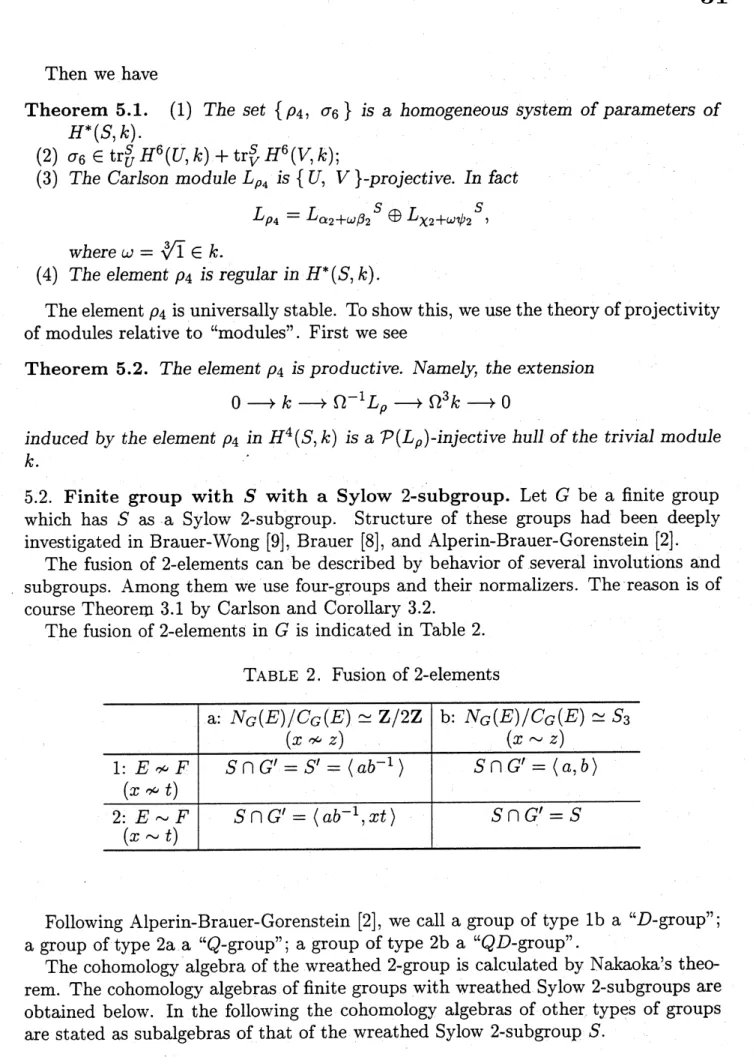
Sylow 2-subgroup. Structure of these groups had been deeply

investigated in Brauer-Wong [9], Brauer [8], and $\mathrm{A}\mathrm{l}\mathrm{p}\mathrm{e}\mathrm{r}\mathrm{i}\mathrm{n}-\mathrm{B}\mathrm{r}\mathrm{a}\mathrm{u}\mathrm{e}\mathrm{r}-\mathrm{G}_{0}\mathrm{r}\mathrm{e}\mathrm{n}\mathrm{S}\mathrm{t}\mathrm{e}\mathrm{i}\mathrm{n}[2]$ .

The fusion of 2-elements

can

be described by behavior of several involutions and

subgroups. Among them we use four-groups and their normalizers. The

reason

is of

course

Theorem

3.1

by Carlson and Corollary 3.2.

The fusion of 2-elements in $G$ is indicated in Table 2.

TABLE 2. Fusion of 2-elements

Following $\mathrm{A}\mathrm{l}\mathrm{p}\mathrm{e}\mathrm{r}\mathrm{i}\mathrm{n}- \mathrm{B}\mathrm{r}\mathrm{a}\mathrm{u}\mathrm{e}\mathrm{r}-\mathrm{G}_{0}\mathrm{r}\mathrm{e}\mathrm{n}\mathrm{S}\mathrm{t}\mathrm{e}\mathrm{i}\mathrm{n}[2]$ ,

we

call

a

group oftype lb

a

“ $D$-group”;

a

group oftype $2\mathrm{a}$

a

“_$Q$-group”;

a group

of type $2\mathrm{b}$

a

“QD-group”.

The cohomology algebra ofthe wreathed 2-group is calculated by Nakaoka’s

theo-rem.

The cohomology algebras offinite

groups

with wreathed Sylow 2-subgroups

are

obtained below. In the following the cohomology algebras of other types of

groups

are

stated

as

subalgebras of that of the wreathed Sylow 2-subgroup $S$.

(1) If$G$ is oftype 1$\mathrm{a}$, then

$H^{*}(G, k)\simeq H^{*}(S, k)$

$=k[\zeta_{1}, \tau_{1}, \zeta_{2}, \nu_{2}, \zeta 3, \nu_{4}]/((_{1}^{2}, \nu_{2}, \zeta 232, \tau\zeta 1, \tau\zeta 2, \mathcal{T}\zeta_{3}, \nu 2\zeta_{1}, \nu_{2}\zeta 3, \zeta 1\zeta 3-\zeta 2\nu 2)$

.

(2) If$G$ is

a

$D$-group, then

$H^{*}(G, k)=k[_{\mathcal{T}}1, \nu 2, \theta_{3}, \rho 4, \theta_{5,6}\sigma]$,

where

$\theta_{3}=\tau_{1}\nu_{2}+\zeta_{1}\zeta_{2}+\zeta_{3},$ $\rho_{4}=\tau_{1}^{4}+\zeta_{2}^{2}+\nu_{4},$ $\theta_{5}=\tau^{3}\nu_{2}+\zeta_{1}\rho_{4}+\zeta_{2}\zeta_{3},$ $\sigma_{6}=(\tau_{1}^{2}+\zeta_{2})\nu_{4}$

(3) If$G$ is

a

$Q$

-group,

th

en

$H^{*}(G, k)=k[(_{1}, \sigma_{2}, \theta 3, \rho_{4}]$,

where

$\sigma_{2}=\mathcal{T}_{1}^{2}+\zeta_{2}$.

(4) If$G$ is a _$QD$-group, then

.

$H^{*}(G, k)=k[\theta_{3}, \rho_{4_{)}5_{)}}\theta\sigma 6]$.

Remark 5.1. The elements $\zeta_{1},$ $\nu_{2}$, and $\zeta_{3}$ above will $\mathrm{b}.\mathrm{e}$ stated in subsection 5.5.

To show that the element$\rho_{4}$ in $H^{4}(S, k)$ is universally stable,

we

show the following

Theorem 5.4. There exists

a

$kG$-module $\overline{X}$

such that

$\overline{X}_{S}=L_{\rho}\oplus(\mathrm{P}^{\mathrm{r}\mathrm{o}}\mathrm{j}\mathrm{e}\mathrm{C}\mathrm{t}\mathrm{i}\mathrm{v}\mathrm{e})$

.

Using Theorem 5.4, Lemma 2.5, and lemma 2.4,

we can

show

Theorem 5.5. There exists

a

productive element $\overline{\rho}$ in $H^{4}(G, k)$ such that

$\mathrm{r}\mathrm{e}\mathrm{S}_{S\overline{\rho}=\rho},$ $L_{\overline{\rho}}=\overline{X}$.

5.3. $QD$-groups. Our proof of Theorem 5.4 is slightly complicated. So

we

sketch

our argument only for $QD$-groups $G$; namely suppose, in this subsection, that the

four-groups $E$ and $F$ are conjugate in $G$ and the quotient group _{$N_{G}(E)/C_{G}(E)$} is

isomorphic with $S_{3}$. Let $H$ be the subgroup of _{$N_{G}(E)$} of index two containing the

centralizer $C_{G}(E)$. We may assume that there exists an element $h$ in $H$ such that

$a^{h}=b_{J}.b^{h}=ab$.

Suppose for the moment that there exits

an

element $\overline{\rho}$in $H^{4}(G, k)$ such that

$\mathrm{r}\mathrm{e}\mathrm{S}_{S\overline{\rho}=\rho}$.

Then

an

indecomposable direct summand $\overline{X}$

of the Carlson module $L_{\rho}\sim$ would have

vertex $U$ and a

source

$L_{\alpha_{2}+\omega\beta_{2}}$ so that

$\overline{X}$

would be the Green correspondent of

an

indecomposable direct summand $X’$ of the Carlson module $L_{\rho’}$ of the restriction

$\rho’=\mathrm{r}\mathrm{e}\mathrm{s}_{N_{G}(E})\overline{\rho}$ with vertex $U$ and a

source

$L_{\alpha_{2}+\omega\beta_{2}}$

.

We write $N=N_{G}(E)$ and

$C=C_{G}(E)$. We know that the centralizer $C_{G}(E)$ has a normal 2-complement:

Let

$\epsilon.=\alpha_{2}+\omega\beta_{2}$

.

Since $C_{G}(E)=U\ltimes O(C_{G}(E))$, the Carlson module$L_{\epsilon}$

can

beextendedto $C=C_{G}(E)$

.

We denote by $L_{C}$ the extension of$L_{\epsilon}$ to $C_{G}(E)$:

$L_{C|U}\simeq L_{\epsilon},$ $L_{C))}|O(c_{G}(E=\mathrm{t}\mathrm{r}\mathrm{i}_{\mathrm{V}}\mathrm{i}\mathrm{a}1$ module.

Because the module $X’$ belongs to the principal $kN$-block, the module $X’$ is

a

direct

summand of the induced module $L_{C^{N}}$. The induced module $L_{C^{N}}$

can

be analyzed

by Clifford theory. First

we

have

$H=\{X\in N|Lx\simeq\xi L_{\epsilon}\}$

.

Thus if$L_{C^{H}}= \sum M_{j}$ is

an

indecomposable decomposition, then the induced modules

$M_{j}^{N}\mathrm{s}$

are

indecomposable and $L_{C^{N}}= \sum M_{j}^{N}$. Indeed the induced module $L_{C^{H}}$

decomposes

as

follows.

Lemma 5.6. For $i=0,1,2$ , let $k_{i}$ be the one-dimension$\mathrm{a}lkH$-module

on

which $U$

acts trivially and the elem

en

$\mathrm{t}h$ acts

as

multiplication by$\omega^{i}$

.

Then the indu$c\mathrm{e}d$module

$L_{C^{H}}$ has

a

decomposition

$Lc^{H}=M0\oplus M_{1}\oplus M2$

ofindecompos

a

$blekH$-modules $M_{0,1}M,$ $M_{2}$ such that

(1) $M_{i|U}\simeq L_{\epsilon},$ $i=0,1,2$ ;

(2) $M_{i}s$

are

periodic ofperiod six,

(3) $M_{i}\simeq M_{0}\otimes k_{i},$ $i=0,1,2$ ;

(4)

$M_{0}/\mathrm{r}\mathrm{a}\mathrm{d}M_{0}=k_{2}\oplus k_{0}$,

soc

$M_{0}=k_{1}\oplus k_{2;}$ $\Omega(M_{0})/\mathrm{r}\mathrm{a}\mathrm{d}\Omega(M_{0})=k_{0}\oplus k_{1}$,

soc

$\Omega(M_{0})=k_{2}\oplus k_{0;}$

(5) $\Omega^{2}(M_{0)}=M_{2}, \Omega^{2}(M_{1})=M_{0},$ $\Omega^{2}(M_{2})=M_{1}$.

The indecomposable $kN$-module $X’$ would be one of$M_{i;}^{N_{\mathrm{S}}}$ we put, say,

$X’=Mi^{N}$.

Since the module $\Lambda’I_{i}^{N}$ would be

a

direct summand of $L_{\rho’}$, the module $M_{i}$ would be

a direct summand of the Carlson module $L_{\rho’’}$ of the restriction $\rho^{\prime/}=\mathrm{r}\mathrm{e}\mathrm{s}_{H}\rho’$

.

Now let

us

return to construction ofthe $kG$-module $\overline{X}$

.

Lemma 5.7. The cohomology$\rho_{4}$ is $N_{G}(E)-S\mathrm{t}\mathrm{a}bl\mathrm{e}$.

Definition 5.3. Let

us

take $\rho’$ in $H^{4}(Nc(E), k)$ such that $\mathrm{r}\mathrm{e}\mathrm{s}_{S\rho’=}\rho$

.

Then

we

have $\rho’=\mathrm{t}\mathrm{r}^{N}s\rho$. We also let $\rho’’=\mathrm{r}\mathrm{e}\mathrm{s}_{H}\rho’$. Then

we

have

Proposition 5.8. The Carlson module $L_{\rho’’}$ has

a

decomposition

$L_{\rho’’}=M\oplus M^{t}$

ofindecomposa$blekH$-modules $M$ and $M^{t}$ such that

(1) $M_{U}\simeq L_{\mathrm{g}}$;

(2) $M^{N_{U}s_{;}}\simeq L_{\epsilon}$

(3) $M$ is periodic of period six,

(4)

$M/\mathrm{r}\mathrm{a}\mathrm{d}M=k_{1}\oplus k_{2}$,

soc

$M=k_{0}\oplus k_{1;}$

$\Omega(M)/\mathrm{r}\mathrm{a}\mathrm{d}\Omega(M)=k_{2}\oplus k0$,

soc

$\Omega(M)=k_{1}\oplus k2$; $\Omega^{2}(M)/\mathrm{r}\mathrm{a}\mathrm{d}\Omega 2(M)=k_{0}\oplus k_{1}$,

soc

$\Omega^{2}(M)=k_{2}\oplus k0$;

(5) For$i\geq 0$

$\Omega^{i+3}(M)/\mathrm{r}\mathrm{a}\mathrm{d}\Omega^{i+3}(M)\simeq\Omega^{i}(M)/\mathrm{r}\mathrm{a}\mathrm{d}\Omega i(M)$ ;

soc

$\Omega^{i+3}(M)\simeq \mathrm{s}\mathrm{o}\mathrm{c}\Omega^{i}(M)$

.

Definition 5.4. Let

$X’=M^{N}$_.

The indecomposable $kN$-module $X’$ has vertex $U$ and

source

$L_{\epsilon}$.

By

our

definition ofthe indecomposable $kN$-module $X’$

we

have

Proposition 5.9. (1) The indecomposa$blekN$-module $X’$ isperio$\mathrm{d}ic$ofperiod six.

(2) $X_{S}’=L\epsilon s$.

(3) The indecomposable $kN$-module $X’$ is

a

direct summand of$L_{\rho’}$.

Using the proposition above and the assumption that the four-groups $E$ and $F$ are

conjugate,

we

obtain

Proposition 5.10. It follows that

$X^{\prime G}s\equiv L_{\rho}$ (mod projective).

We can now define the $\dot{k}G$-module $\overline{X}$

.

Definition 5.5. Let

$\overline{X}$

be

a

Green correspondent of$X’$ with respect to $(G, U, N_{G}(E))$.

By

means

ofPropositions 5.9,

5.10

and the properties ofthe Greencorrespondence

we

see

that the $kG$-module $\overline{X}$

is the desired

one.

Theorem 5.11. We have

(1) the $kG$-module $\overline{X}$

isperiodic of period six;

(2)

$X^{;G}=\tilde{X}\oplus(\mathrm{P}^{\mathrm{r}\mathrm{o}}\mathrm{j}\mathrm{e}\mathrm{C}\mathrm{t}\mathrm{i}\mathrm{V}\mathrm{e})$;

(3)

$\tilde{X}$

$\rho’=\rho^{N}$ $X’=M^{N}$

$\rho^{\prime/}=\rho_{H}’$ $L_{\rho’’}=M\oplus M^{t}$

$L_{\rho}$ $\rho$ $L_{C}$

$L_{\epsilon}$ $\epsilon$

Remark

5.2.

When the $\mathrm{f}\mathrm{o}\mathrm{u}\mathrm{r}$

’-groups

$E$ and $F$

are

not conjugate in $G$, the $kG$-module

$\overline{X}$

in Theorem

5.4

is not indecomposable.

5.4.

Relative injective hull of the trivial module. We

resume

our

situation that

$G$ is a finite

group

with wreathed Sylow 2-subgroup $S$

.

The element $\overline{\rho}_{4}$ is productive

by Theorem 5.5. The $L_{\overline{\rho}}$-injective hull

$0arrow k_{G}arrow\Omega^{-1}(L_{\overline{\rho}})arrow\Omega^{3}(k_{G})arrow 0$

gives

us

much information about the cohomology algebra. First

we can

deduce the

following theorem from Theorem

3.3.

Theorem 5.12. The element $\sigma_{6}$ is universallystable. Namely thereexists

an

element

$\overline{\sigma}_{6}\in H^{6}(G, k)$ such that

$\mathrm{r}\mathrm{e}\mathrm{s}_{S}\tilde{\sigma}_{6}=\sigma_{6}$.

Consequently the set

$\{\rho_{4}, \sigma_{6}\}$

is

a

homogeneo

us

system of$p$

aram

eters for $H^{*}(G, k)$ for every $G$

.

Second

we can

obtain dimension formulae for the cohomology

groups

$H^{*}(G, k)$

.

Applying the cohomology functor $\mathrm{E}\mathrm{x}\mathrm{t}_{kG}(-, k)$ to the extension

$0arrow k_{G}arrow\Omega^{-1}L_{\rho}\simarrow\Omega^{3}k_{G}arrow 0$,

we

obtain the short exact sequences

$0arrow \mathrm{H}\mathrm{o}\mathrm{m}_{kG}(\Omega 3k, k)arrow \mathrm{H}\mathrm{o}\mathrm{m}_{kG}(\Omega^{-}1L\sim k\rho_{4}’)arrow 0$,

$0arrow \mathrm{E}_{\mathrm{X}\mathrm{t}_{kG}^{n}}(k, k)arrow \mathrm{E}\mathrm{x}\mathrm{t}_{k^{+}}^{n}(ck1\Omega 3, k)arrow \mathrm{E}\mathrm{x}\mathrm{t}_{k}^{n+1}c(\Omega-1L^{\sim k}\rho_{4}’)arrow 0$, $n\geq 0$

.

In particular

we

_ha.ve

a

$\mathrm{f}_{\mathrm{o}\mathrm{r}\mathrm{m}\mathrm{u}}....1\mathrm{a}$

and

we can

compute $\dim \mathrm{E}\mathrm{x}\mathrm{t}n(kGL_{\rho_{4}}^{\sim,k})$ by

our

construction of the module $\tilde{X}=L_{\rho}^{\sim}$

.

For example, if$G$ is

a

_$QD$-group, then

$\dim \mathrm{E}\mathrm{x}\mathrm{t}_{k}n_{G(L\rho 4}\sim,$

$k)=$

We

can

also calculate $\dim \mathrm{E}_{\mathrm{X}\mathrm{t}^{n}}(kGk, k),$ $n=1,2,3$,

so

that

we

obtain dimension

formulae for $H^{*}(G, k)$

.

We have obtained

a

system of parameters $\{\rho_{4},\sigma_{6}\sim\sim\}$ and established dimension

formulae for the cohomology

groups

$H^{*}(G, k)$

.

We have to get generators of the

cohomology algebras over the subalgebra $k[\rho_{4},\overline{\sigma}_{6}\sim]$.

5.5. Generators of Cohomology Algebras. First let

us

state generators of the

cohomology algebra of the wreathed 2-group $S$. The cohomology algebra $H^{*}(S, k)$

has $\{\sigma_{2}(=\tau_{1}^{2}+(2), \rho_{4}\}$

as a

system of parameters. Hence we

can

take generators

ofdegree up to 4. In fact, $H^{*}(S, k)$ is generated

over

the subalgebra $k[\sigma_{2}, \rho_{4}]$ by $\tau_{1}$,

which

was

defined in Section 2, and the elements $\zeta_{1,2}l^{\text{ノ}},$ $\zeta 3\in H^{*}(S, k)$. To state these

elements, let $\alpha_{1}\in\inf^{U}H^{1}(U/\langle b\rangle, k)$; and let

us

define .

$\zeta_{1}=\mathrm{t}\mathrm{r}_{U}^{s}\alpha 1\in H^{1}(S, k)$,

$\nu_{2}=\mathrm{n}\mathrm{o}\mathrm{r}\mathrm{m}_{U}^{S}\alpha_{1}\in H^{2}(S, k)$,

$\zeta_{3}=\mathrm{t}\mathrm{r}_{U}^{S}(\alpha_{1}\alpha_{2})\in H^{3}(S, k)$

.

When the four-groups $E$ and $F$

are

not conjugate in $G$, the cohomology algebras

$H^{*}(G, k)$ and $H^{*}(N_{G}(E), k)$

are

isomorphic. This

can

be

seen

by comparing the

di-mensions of the cohomologygroups. On the other hand, when$E$ and $F$

are

conjugate,

one can

take

an

element $g_{0}\in C_{G}(C)$ such that $E^{\mathit{9}0}=F$ and $U^{\mathit{9}0}\cap S=V$

.

Then

we

can

determine the stable elements by considering the subspaces

$\{\xi\in H^{n}(S, k)|\xi^{\mathit{9}0}V=\xi_{V}\}$, $n\leq 4$.

Of

course

the element $g_{0}$ aboveplays

an

important rolethroughout in

our

investigation

for those groups in which $E$ and $F$

are

conjugate.

REFERENCES

[1] A. Adem and R. Milgram, The mod 2 cohomology rings

_of

rank 3 simple groups

are Cohen-Macaulay, Prospects in topology (Princeton) (F. Quinn, ed.), Ann.

Math. Studies, vol. 138, Princeton Univ. Press, 1995, pp. 3-12.

[2] J. L. Alperin, R. Brauer, and D. Gorenstein, Finite groups with quasi-dihedral

and wreathed Sylow 2-subgroups, ’bans. Amer. Math. Soc. 151 (1970), 1-261.

[3] –, Finite simple groups

of

2-rank two, Scripta Math. 29 (1973),

191-214.

[4] T. Asai, A dimension

_{formula for}

the cohomology rings

_of

_finite

groups with

dihedral Sylow 2-subgroups, Comm. Algebra 19 (1991), 3173-3190.

[5] T. Asai and H. Sasaki, The mod 2 cohomology algebras

_{of finite}

groups with

[6] D. J. Benson, Representations and cohomology II.. Cohomology

_of

groups and

modules, Cambridge studies in advanced mathematics, vol. 31, Cambridge

Uni-versity Press, Cambridge, 1991.

[7] D. J. Benson and J. F. Carlson, Diagrammatic methods

_for

the modular repre-sentations and cohomology, Comm. Algebra 15 (1987),

53-121.

[8] R. Brauer, Character theory

_of

_finite

groups with wreathed Sylow 2-subgroups, J.

Algebra 19 (1971),

547-592.

[9] R. Brauer and W. J. Wong,

Some

properties

_of

_finite

groups with wreathed Sylow

2-subgroups, J. Algebra 19 (1971), 263-273.

[10] J. F. Carlson, Depth and

_transfer

maps in the cohomology

_of

groups, Math. Z.

218 (1995),

461-468.

[11] –, Modules and group algebras, Lectures in Mathematics, ETH Z\"urich,

Birkh\"auser, $\mathrm{B}\mathrm{a}\mathrm{s}\mathrm{e}\mathrm{l}/\mathrm{B}\mathrm{o}\mathrm{s}\mathrm{t}\mathrm{o}\mathrm{n}/\mathrm{B}\mathrm{e}\mathrm{r}\mathrm{l}\mathrm{i}\mathrm{n}$ ,

1996.

[12] L. Evens, The cohomology

_of

groups, Oxford $\grave{\mathrm{M}}$

athematics Monograph, Oxford

University Press, New York,

1991.

[13] L. Evens and S. Priddy, The ring

_of

universally stable

_element.s,

Quart.

’J.

Math.

Oxford (2) 40 (1989),

399-407.

[14] S. Fiedorowizc and S.

Priddy,

Homology

_of

classical groups over

_{finite fields}

and

their associated

_infinite

loop spaces, Springer Lecture Notes in Math., vol. 674, Springer-Verlag, $\mathrm{B}\mathrm{e}\mathrm{r}\mathrm{l}\mathrm{i}\mathrm{n}/\mathrm{N}\mathrm{e}\mathrm{w}\mathrm{Y}_{0}\mathrm{r}\mathrm{k}/\mathrm{H}\mathrm{e}\mathrm{i}\mathrm{d}\mathrm{e}\mathrm{l}\mathrm{b}\mathrm{e}\mathrm{r}\mathrm{g}$ ,

1978.

[15] D. Gorenstein, Finite groups, Harper&Row, Publishers, New York, 1968.

[16] D. Gorenstein and J. H. Walter, The characterization

_{of finite}

groups with

dihe-dral sylow 2-subgroups, I, II, III, J. Algebra 2 (1965), 85-151, 218-270, 334-393.

[17] R. Kn\"orr, Relative projective covers, Proc. Symp. Modular Representations of

Fi-nite Groups, Various Publication Series, vol. 29, Aarhus University, 1978, pp.

28-32.

[18] I. J. Leary, The mod-p cohomology rings

_of

some $p$-groups, Math. Proc.

Cam-bridge Philos. Soc. 112 (1992),

no.

1, 63-75.

[19] R. Lyons, A characterization

_of

$U_{3}(4)$, bans. Amer. Math. Soc. 164 (1972),

371-387.

[20] J. Martino, Stable splittings

_of

the Sylow 2-subgroup8

_of

$\mathrm{S}\mathrm{L}_{3}(\mathrm{F}_{q}),$

q-odd,

Ph.D.

thesis, Northwestern University,

1988.

[21] J. Martino and S. Priddy,

_{Classification}

_of

BG

_for

groups with dihedral or

quater-nion Sylow 2-subgroups, J. Pure Appl. Algebra 73 (1991),

13-21.

[22] H. Nagao and Y. Tsushima, Representations

_of

_finite

groups, Academic Press,

New York, London, 1989.

[23] T. Okuyama, A generalization

_of

projective

covers

_of

modules over group algebras,

unpublished manuscript.

[24] H. Sasaki, The mod 2 cohomology algebras

_{of finite}

groups with

semid\‘ih’edral

Sylow 2-subgroups, Comm. Algebra 55 (1994),

243-275.

[25] M. Tezuka and N. Yagita, The

_mod\ldots

p cohomology

_of

$\mathrm{G}\mathrm{L}_{3}(\mathrm{F}_{p})$, J. Algebra 81

(1983),

295-303.

[26] M. Tezuka and N. Yagita., On odd prime components

_of

cohomologies sporadic

simple groups and the rings

_of

universal stable elements, J. Algebra 186 (1996),