JAIST Repository: A new Interconnection Network that achieves High Performance for Many-Core Processors

(1)

JAIST Repository

https://dspace.jaist.ac.jp/

Title A new Interconnection Network that achieves High Performance for Many-Core Processors

Author(s) FAISAL, FAIZ AL Citation

Issue Date 2015-03

Type Thesis or Dissertation Text version author

URL http://hdl.handle.net/10119/12637 Rights

Description Supervisor: Yasushi Inoguchi, School of Information Science, Master

(2)

List of Figures

2.1 Architecture of MESH Network [9] . . . 13

2.2 Architecture of Torus Network [9] . . . 13

2.3 Architecture of TOFU Network [11] . . . 14

2.4 Architecture of 5D-Torus Network [12] . . . 15

2.5 Architecture of TESH Network [5] . . . 16

2.6 Architecture of TTN Network [6] . . . 16

2.7 Architecture of STTN Network [7] . . . 17

2.8 Packet transmission using 2 virtual channels[13] . . . 20

3.1 A (4× 4 × 4) Basic Module of 3D-TESH Network . . . 22

3.2 A (4× 4 × 4) Basic Module of 3D-TESH(2,3,1) Network . . 23

3.3 Higher-level of Interconnection for 3D-TESH Network . . . 25

3.4 Routing Path for 3D-TESH Network . . . 34

4.1 Diameter Performance for Various Networks . . . 37

4.2 Average Distance for Various Networks . . . 39

4.3 Cost Performance for Various Networks . . . 39

4.4 Bisection Bandwidth for Various Networks . . . 40

5.1 Link Power Analysis for Various Networks . . . 43

5.2 Router Power Analysis for Various Networks . . . 44

5.3 Schematic showing board-level electrical interconnects. This figure is obtained from reference [20] . . . 44

5.4 Power comparison for oﬀ-chip interconnect. This graph is ob-tained from reference [20] . . . 46

5.5 Power comparison for various networks(64 on-chip nodes) . . . 47

5.6 Uniform traﬃc with 2 cycle wire delay . . . 50

5.7 Matrix Transpose traﬃc with 2 cycle wire delay . . . 50

(5)

5.9 Perfect Shuﬄe traﬃc with 2 cycle wire delay . . . 51

(6)

List of Tables

3.1 Generalization of 3D-TESH Network . . . 24

3.2 Example of various levels of 3D-TESH network . . . 24

3.3 Generalization of number of links at various levels of 3D-TESH 27

3.4 Example of required number of links at various levels of networks 27

4.1 Node Degree of Various Networks . . . 36

4.2 Calculated Formulation of Diameter for 3D-TESH Network. . 38

4.3 Arc Connectivity for Various Networks . . . 40

5.1 Simulation condition for level-1 3D-TESH network . . . 43

5.2 Power estimation for various networks(2mm link length, 1

vir-tual channel & 64 nodes) . . . 43

5.3 Board trace parameters and the corresponding SPICE

param-eters used for dielectric and skin eﬀect. This table is obtained

from reference [20]. . . 45

(7)

Abstract

Next generation high performance computing (HPC) highly depends on the massively parallel computers (MPC). The overall performance of a massively parallel computer system is heavily affected by the interconnection network and its processing nodes. Continuing advances in VLSI technologies promise to delivering more power to individual nodes. But the on-chip interconnec-tion networks consume 50% of the total power and off-chip bandwidth is limited to the maximum number of possible out going physical links. On the other hand, low performance of communication network degrades the parallel system. Hence it is important to find a suitable interconnection network with the existing technologies and at the same time it is also important to evalu-ate the network performance. In this research proposal, we like to introduce a new interconnection network that could reduce those problems (like- high power consumption, longer wire length, low bandwidth issue and etc.) and also like to measure the static and dynamic communication performance of our newly introduced interconnection network, comparing the performance results with other networks at different levels of hierarchy such as inter-chips, inter-nodes and inter-cabinets.

(8)

Acknowledgments

First of all, I would like to express my deepest gratitude to my supervisor, Professor Yasushi Inoguchi for his great support and eﬀective advise during my research period. His guidance helped me to find the correct direction of my research. His constant inspiration and encouragement allow me to reach the final goal of this research.

Secondly, I like to express my sincere thanks to Assistant Professor Yukinori Sato (School of Information Science, Japan Advanced Institute of Science and Technology) and Assistant Professor M.M. HAFIZUR RAHMAN (De-partment of CS, KICT, IIUM) for their kind supports during my research period.

Then, I like to express my gratitude to second supervisor Associate Professor Kiyofumi Tanaka for his cordial advices during my research.

I also wish to express my honor to my sub-theme supervior Associate Pro-fessor Masato Suzuki and ProPro-fessor Mineo Kaneko for their valuable advices and suggestions.

I am eagerly acknowledge the Japan Educational Exchanges and Services (JEES) for granting me the ”2013 NTT DOCOMO Scholarship for

Appli-cants Residing Abroad” which makes my study and life feasible in Japan.

And also acknowledge the ”Research Grants for JAIST Students” which al-lows me to present my research work in international conference.

Finally, I like to give my sincere acknowledgments to my family members for their huge support and patience; to my father, my mother and also to my spouse.

(9)

Chapter 1 Introduction

1.1 Background

High performance computer (HPC) is the increased demand for next gener-ation of computers. Sequential computers fails to meet this demand and already reached to the saturation point due to the scaling diﬃculties of uniprocessor architectures. Hence the need for massively parallel computers (MPC) is increasing day by day. Massively parallel computers with thou-sand of nodes have been commercially available with tera-flops performance and eﬀorts have been made to build MPC systems with millions of nodes for peta-flops or even for exa-flops performance. To facilitate the millions of node, interconnection networks are the key elements [1]. Interconnection network acts as a path between one node to another. Considering millions of nodes, the large diameter of conventional interconnects is completely in-feasible. On the other hand, to jump into the next level there is few key constraints that limit network performance, cost-performance ratio, power consumption, throughput and latency [2].

In the future intuitive, flexible and highly interactive parallel computers with massive computation power will replace the recent sequential comput-ers having small computation power. Parallel computcomput-ers will not only be an important factor for day-to-day life, will also be a major shortcut for next generation technologies. Even now a day, parallel computer has become an integral part of society. Sectors like- Banking, Education system, Military, communication and even in research fields, usages of parallel computer has already been boosted up and removed all the traditional equipment. But the

(10)

problem resides for parallel computer like- supercomputers is its processing power, memory, inter-communication between the CPUs, power consump-tions and the cooling systems.

1.2 Problem Statement

One of the main constraints for MPC systems is the suitable interconnection network that could be scaled up to millions of nodes with small diameters. Next is the cost-performance issue, increased outgoing link from each node increases the total cost of the network. Interconnection links consume the most of the power; shorter link consumes smaller power where as longer links consumes more power. Even according to the advancement of current tech-nology to build a one exa-flop system, it needs close to 1000MW of electrical power, which indeed a major constraint for next generation computers. And also it is always desirable an interconnection network with low latency and high throughput for high network performance.

1.3 Objective

Hierarchical Interconnection networks (HIN) [3] are cost-eﬀective way to in-terconnect a large processing system. Even lots of hypercube based hierarchi-cal interconnection networks have also been available; but for MPC systems, the number of physical links is a major concern. With the early researches, TORUS networks shows better performance than the MESH network due to the tori connections but consumes more power than the MESH network due to the increased connections and even the total cost increases for the in-creased links. One of the recently used network is the TOFU interconnection network [4], which requires 10 outgoing links for each node; causing more cost than the other networks and even the scaling at higher level causes low performance issues. Hence it is important to find a new interconnection net-work with concerning the key constraints and improved netnet-work performance as well as reducing the overall power consumption than the other existing networks.

(11)

1.4 Approach

High computation power is the great challenge and also the increased de-mand for next generation computers. Two-dimensional (2D) networks were the main focus for recent studies; with the increase of cores, traditional 2D networks are no longer eﬃcient for many-core processors. Even it consumes more power and shows lower performance than the 3D networks. Hence it is important to find a new interconnection network, which is suitable for next generation interconnection network with reduced power and shorter connects. Routing plays a vital role for the overall performance of the inter-connection networks. Dimension-order routing has been popular for MPC systems due to its minimal hardware requirements and allows the design of simple and fast routers. Routing for MESH and TORUS uses the dimension-order routing. Hence it is also important to find a suitable routing logic for the new interconnection network.

1.5 Scope of the Thesis

Network topology aﬀects the performance metrics. In previous researches, HIN networks (like- TESH [5], TTN [6] and STTN [7]) show better static network performance than the conventional MESH and TORUS networks. It is being expected for the interconnection network with low cost, low degree, low congestion, high connectivity and high fault tolerance. With fixed rout-ing logic, it is important to measure the static network performance of new interconnection network to compare the performance result with the other conventional networks. Evaluating the static network performance consists of measuring the below

parameters-1. Diameter. 2. Average Distance.

3. Node Degree. 4. Cost. 5. Power Consumption.

The actual performance of the network can be found through the dynamic communication performance. Low latency and high network throughput are desirable for any interconnection network [8]. To compare the new network dynamic communication performance with the TORUS, MESH and even with the recent networks, it is also needed to find performance results with the common parameters for new network and others. Uniform traﬃc pat-tern will help to compare the dynamic performance of new network with the

(12)

existing networks. And the non-uniform load distribution will be helpful to observe the networks maximum tolerance capabilities. Evaluating the dy-namic communication performance of new interconnection network consists of measuring the below

parameters-1. Network Latency 2. Network Throughput

1.6 Organization of the Thesis

At the end of this chapter the rest of the paper is organized as follows. In chapter 2, we deal with the relative conventional interconnection networks, their architecture and also the other hierarchical interconnection like- TESH, TTN and STTN with their architectural interconnections. In chapter 3, we deal with the concept of 3D Tori connected mESH Network (3D-TESH), his architecture, the addressing and the routing algorithm of 3D-TESH. In chapter 4, we evaluate the static network performance of 3D-TESH with respect to other conventional network performance. Chapter 5 presents the evaluation of the dynamic network performance of 3D-TESH with respect to other conventional network performance. Chapter 6 presents the conclusion of this research work and gives some direction of future works.

(13)

Chapter 2 Related Works

2.1 Introduction

Massively Parallel Computes (MPC) highly depend on the interconnection networks. But interconnection network with large diameter is completely infeasible. Hierarchical Interconnection network (HIN) are cost-eﬀective way to interconnect a large processing system. Even lots of hypercube based hi-erarchical interconnection networks have also been available; but for MPC systems, the number of physical links is the major concern. A MPC system with small number of outgoing links is cost eﬀective and desirable. To move into the next generation systems, key constraints will be the network perfor-mance, cost-performance ratio, power consumption, throughput and latency [2]. In this research, we like to develop a new interconnection network from the viewpoint of reduced power consumption; whereas one of the possible candidates for interconnection network can be the hierarchical interconnec-tion network.

2.2 Various types of Interconnection Networks

2.2.1 MESH Network

Mesh [9] is one of the k-ary n-cube networks, which is easy to layout in on-chips due to its regular and equal-length links. It has high path diversity i.e., there is many ways to reach from one node to another. Mesh has been

(14)

Latency is O(sqrt(N)) and has O(N) cost. Figure 2.1 shows the architectural interconnect for 2D-Mesh network.

Figure 2.1: Architecture of MESH Network [9]

2.2.2 TORUS Network

Mesh is not symmetric on edges hence its performance very sensitive to place-ment of task on edge vs. middle. Torus [9] network avoids this problem. It has higher path diversity (& bisection bandwidth) than mesh network. It requires higher cost and harder to layout on-chip and unequal link lengths. Figure 2.2 shows the node level interconnections for 2D-Torus network.

Figure 2.2: Architecture of Torus Network [9]

(15)

2.2.3 TOFU Network

TOFU interconnection network has been adopted by the Fujitsu K computer and already achieved 10.51 petaflops performance requiring power consump-tion of 12.6 MW [10]. TOFU network has 6 dimensional mesh/torus in-terconnect. 10 links are used for inter-node connection of TOFU network, where 6 links are scalable for connecting 3D-torus interconnect and another 4 links are fixed sized connecting 3D-mesh/torus topology. Figure 2.3 shows the interconnecting structure of TOFU network.

Figure 2.3: Architecture of TOFU Network [11]

2.2.4 5D-TORUS Network

5D-Torus network shows excellent performance for the MPI-type communi-cations. In 5D-Torus network, one node is connected with 10 neighboring nodes. Recently, 5D-Torus network has been adopted in IBM Blue Gene/Q super-computer. Though 5D-Torus and Tofu interconnect uses same number of outgoing links, 5D-Torus shows better performance over the TOFU inter-connect due to the greater over-provisioning of links and greater fail-proof resiliency by resulting the greater complexity and cost. Figure 2.4 shows the 5D-torus interconnect between the various nodes.

2.2.5 Hierarchical Interconnection Networks (HIN)

2.2.5.1 Tori-connected mESH (TESH) Network

The Tori-connected mESH (TESH) [5] Network is a hierarchical intercon-nection network consisting of Basic Modules (BM) that are hierarchically

(16)

Figure 2.4: Architecture of 5D-Torus Network [12]

interconnected to form a higher level network with multiple lower level

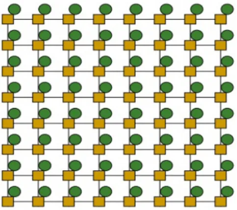
net-works. The BM of the TESH network is a 2D-mesh network of size (2m×2m_).

BM refers to a Level-1 network. Higher level TESH networks are built by re-cursively interconnecting immediately lower level subnetworks in a 2D-torus fachion. A higher-level network is built using a 2D-toroidal connection among

(22m) immediate lower level subnetworks. If m = 2, the size of the BM is (4

× 4), and similarly if m = 3 then the size of the BM will be (8 × 8) [5]. A

BM of (4× 4) is shown in Figure 2.5. As shown in the figure, the BM has

some free ports in the periphery for higher level interconnection. All ports of the interior Processing Elements (PEs) are used for intra-BM connections. All free ports of the exterior PEs, either one or two, are used for inter-BM connections to form higher level networks.

2.2.5.2 Tori-connected Torus Network (TTN)

Tori connected Torus Network (TTN) [6] is also a hierarchical interconnection network. The lowest level of TTN is the Level-1 network defined as the basic module. Multiple basic modules (BM) are hierarchically interconnected to

form a higher level TTN network. A (2m× 2m) BM consists of a 2D-torus

network of 22m _{processing elements (PE) having 2}m _{rows and 2}m _columns,

where m is a positive integer. Figure 2.6 shows the BM for TTN with m =

2, which defines the size of BM as (4 × 4). Each BM has 2m+2 free ports

(17)

Figure 2.5: Architecture of TESH Network [5]

intra-BM level and rest of the free-ports at the exterior nodes, either one or two, are used for inter-BM connections to form higher level networks.

Figure 2.6: Architecture of TTN Network [6]

2.2.5.3 STTN Network

The Symmetric Tori connected Torus Network (STTN) [7] is a hierarchical interconnection network, whose lowest level of network is the Level-1 network defined as the basic module. Multiple basic modules (BM) are hierarchically

interconnected to form a higher level network. A (2m_{× 2}m_{) BM consists of}

(18)

columns, where m is a positive integer. Figure 2.7 depicts the basic

mod-ule for STTN with m = 2, which defines the size of BM as (4 × 4). Each

BM has 2m+2 free ports at the contours for higher level interconnection. All

ports of the interior nodes are used for intra-BM level. All free-ports of the exterior nodes, either one or two, are used for inter-BM connections to form higher level networks. Higher level networks for STTN are built by the

recursive interconnection (22m_{) of the immediate lower level subnetworks.}

Considering (m = 2) a Level-2 STTN network can be formed by

intercon-necting (22×2) = 16 BMs. Similarly, a Level-3 network can be formed by

interconnecting 16 Level- 2 sub-networks.

Figure 2.7: Architecture of STTN Network [7]

2.3 Importance of multi-dimensional network

(3D-TESH)

Interconnection network consists of multiple nodes communicating with oth-ers directly or indirectly. In direct networks, point to point links intercon-nection is used and in indirect conintercon-nection, communication is carried through some switches. Already large numbers of interconnection network have been proposed, ranging from conventional to hierarchical interconnects. With in-creased demand of high computational power, two dimensional (2D) inter-connection networks are no longer suﬃcient for many-core processors due

(19)

to the limited capacity for single core processors. As the multi-dimensional interconnection has the advantages of shorter global interconnects, high per-formance & low power consumption, this is the key motivation for us to consider a multi-dimensional network. On the other hand, according to the previous researches hierarchical networks shows better performance than the conventional networks. Hence in this research plan, we have considered a new multi-dimensional hierarchical interconnection network(3D-TESH) with two dimensional higher-level of interconnections.

Regarding the consideration of two dimensional interconnection for the higher level networks, is based upon the complexity of the network. If we have considered a three or more dimensional interconnection network at the higher level, the network size will be increased much more than two dimensional interconnect. Hence the wiring complexity and the power consumption will also be increased. But in this research plan, we are trying to find a new interconnection network that will require less power consumption and show better network performance. Hence we have considered a two dimensional interconnect at the higher level of 3D-TESH network.

2.4 Virtual Channels

Virtual channels are very important factor for the analysis of dynamic com-munication performance evaluation. The most common method for imple-menting separate buﬀering resources at each input port is known as virtual channels (VC). The hardware cost increases with the number of virtual chan-nels increases. The unconstrained use of virtual chanchan-nels is cost-prohibitive in parallel systems. Therefore, a deadlock-free routing with minimum num-ber of virtual channels is expected. Virtual channels are used to solve the deadlock avoidance problem, but they can be also used to improve network latency and throughput. Figure 2.8 illustrates two model situations:

”as-sume packet P0 arrived earlier and acquired the channel between the two

routers first. In absence of virtual channels, packet P1 arriving later would

be blocked until the transmission of P0 has been completed. Assume now

that physical channels implement two virtual channels. Upon arrival of P1,

the physical channel is multiplexed between them on a flit-by-flit bases and both packets proceed with half speed. Using of 2 virtual channels for the above situation, is based upon the below two

(20)

packet of size of few flits. Then this scheme allows P1pass through both

routers while P0 is slowed down for a short time corresponding to the

transmission of few packets.

• Assume that P0 is temporarily blocked downstream from the current

router. Then P1 can proceed at the full speed of the physical channel”

[13].

Deadlock is fatal for an interconnection network. When resources (buﬀers or channels) are occupied by deadlocked packets, other packets are also blocked by these resources and finally paralyzes network operation. To pre-vent this situation, networks must either use deadlock avoidance or deadlock recovery. Almost all modern network use deadlock avoidance, usually by imposing an order for the resources and insisting that packets acquire these resources in order. On the other hand, one of the common method to avoid the deadlocks by using the virtual channels. Here, lemma 1 and lemma 2 describes the required number of virtual channels for various conventional networks.

”Lemma 1: If the message is routed in the z → y → x direction in a

3D-torus/3d-mesh network, then the network is deadlock free with 2 virtual channels” [3].

”Lemma 2: If the message is routed in the y → x direction in a 2D-torus

(21)

Figure 2.8: Packet transmission using 2 virtual channels[13]

In this research plan, we have also used 6 virtual channels for our dynamic communication performance. We have used Topaz NoC simulator [14] to simulate on-chip network performance with the 64 nodes. Please find the Appendix B for the virtual channel implementation code of Topaz simulator.

2.5 Summary

In this chapter, we have introduced few interconnection networks which is used for the performance comparison in this thesis. MESH and TORUS are conventional interconnection networks. Even today most of the modern super-computers uses conventional interconnection networks. Blue Gene/Q super-computer built by IBM corporation uses the 5D-Torus interconnection network. On the hand, HIN is the one of the possible solution for high cost-performance and low power consumption issues due to reduced number of outgoing link from diﬀerent levels of hierarchies. Here, we have introduced three HIN networks as- TESH, TTN, STTN; their basic architecture and also explained the importance of 3D-TESH network in the field of next generation of supercomputers.

(22)

Chapter 3 Network Architecture

3.1 Introduction

Network topology refers to the static arrangement of inter-links and nodes in an interconnection network. Network topology plays a vital role in a multi-processor system because routing strategy and static network perfor-mance heavily depends on the network topology. Current MPCs with about millions of nodes already reached into 10 peta-flops performance and eﬀorts been made for exa-scale performance. Network topology is the main factor for the next generation exa-scale system as the on-chip interconnection net-works consume 50% of the total power and oﬀ-chip bandwidth is limited to the maximum number of possible out going links. In this chapter, we de-scribe the architectural details of a new hierarchical interconnection network named as 3D-TESH network, higher level connection for 3D-TESH, the node addressing and finally the message routing algorithm for 3D-TESH network.

3.2 Architecture of 3D-TESH

Hierarchical interconnection networks (HINs) [15] are a cost-eﬀective way to interconnect a large number of nodes. 3D-TESH is a HIN consists of basic modules (BMs) that are hierarchically interconnected for higher levels.

Definition: A 3D-TESH(m, L, q) network, by definition is built using 2m

number of 2D-TESH(2m × 2m) basic modules, where m is a positive integer,

(23)

In 3D-TESH, a BM is similar to 3D-mesh network consists of (2m × 2m ×

2m) connected processing elements (PEs) having (2m) rows and (2m × 2m)

columns. Figure 3.1 shows the BM for 3D-TESH with m = 2 which defines

the size of the BM as (4 × 4 × 4). Similarly, if m = 3, then the size of the

BM becomes (8 × 8 × 8) network with 512 nodes.

Figure 3.1: A (4 × 4 × 4) Basic Module of 3D-TESH Network

Lemma 1: Each (2m× 2m× 2m) 3D-TESH BM has 22m+2 free ports for its higher level of interconnections.

Lemma 1 defines the number of free ports for the higher level intercon-nections of 3D-TESH network. In 3D-TESH network for each higher level of

interconnection, a BM uses 2m _{× 4 × (2}q_{) = 2}m+q+2 _{of its free links, where}

2(2m+q_{) free links for vertical interconnections and 2(2}m+q_{) free links for}

horizontal interconnections. Here, q ∈ 0, 1, ..., m defined as the inter-level

connectivity. q = 0 leads to the minimum inter-level connectivity, whereas q = m leads to the maximum inter-level connectivity. As from the figure 3.1,

a (4 × 4 × 4) BM has 22×2+2 = 64 free ports. if we choose m = 2 and

q = 0, then (22+0+2_{) = 16 of the free ports and their associated links are}

used for each higher level interconnection, 8 for horizontal and 8 for vertical connection. However, if the value of L is 2 or 3, the number of vertical in, vertical out, horizontal in, horizontal out connections are more than four, this means that the inter-level connectivity (q) is increasing. Similarly, if m

(24)

= 2 and L = 3, then 8 links can be used for each vertical in, vertical out, horizontal in, horizontal out connections, when q = 1. Figure 3.2 shows the 3D-TESH(2,3,1) interconnections.

Figure 3.2: A (4 × 4 × 4) Basic Module of 3D-TESH(2,3,1) Network

3.3 Higher-level Networks of 3D-TESH

Higher level of 3D-TESH network is built by the recursive interconnection of the immediate lower level of sub-networks. Figure 3.3 shows the higher-level interconnection for 3D-TESH. A Level-2 network can be formed by

(22×2) 16BMs (16 level-1 3D-TESH network). Similarly, a level-3 3D-TESH

network can be formed by interconnecting 16 level-2 sub-networks. As we have considered m is 2, then the number nodes at level-2 network can be

defined by N = (22mL× 2m). Hence number of nodes at level-2 network is

N = (28 _{× 2}2_{) = 1024.}

The maximum level for 3D-TESH can be built by a (2m× 2m× 2m_{) BM}

is Lmax = 2m−q + 1. If inter-level connectivity, q = 0 & m = 2, Lmax=

5; Level-5 is the highest possible level. The maximum number of nodes

in each level of network can be defined as N = (22mL × 2m_{). If m = 2}

& L = 2, then N = 1024. Similarly, a level-3 3D-TESH network will be

consists of N = 22×2×3_{× 4 = 16384 nodes, which is equal to 16 level-2}

(25)

Network, whereas table 3.2 compares the various levels of 3D-TESH network for m = 2 with the diﬀerent inter-connectivity.

Table 3.1: Generalization of 3D-TESH Network

Basic Module inter-connectivity Max Levels Number of Nodes

(2m× 2m× 2m₎ _q _L

max = 2m−q+ 1 NL = (22mL× 2m)

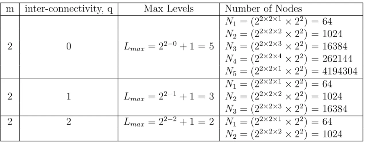
Table 3.2: Example of various levels of 3D-TESH network

m inter-connectivity, q Max Levels Number of Nodes

N1 = (22×2×1× 22) = 64 N2 = (22×2×2× 22) = 1024 2 0 Lmax= 22−0+ 1 = 5 N3 = (22×2×3× 22) = 16384 N4 = (22×2×4× 22) = 262144 N5 = (22×2×1× 22) = 4194304 N1 = (22×2×1× 22) = 64 2 1 Lmax= 22−1+ 1 = 3 N2 = (22×2×2× 22) = 1024 N3 = (22×2×3× 22) = 16384 2 2 Lmax= 22−2+ 1 = 2 N1 = (22×2×1× 22) = 64 N2 = (22×2×2× 22) = 1024

3.4 Number of Channels at Various Levels of

3D-TESH

Larger scaling for supercomputers can make the total cable length enormous e.g., up to thousands of kilometers. Recent high-radix switches with dozens of ports make switch layout and system packaging more complex [16]. The recent K-computer requires cable length near about one thousand kilometers. This section of the paper defines the required number of inter-links between the diﬀerent layers of 3D-TESH network and also compares result with other networks. Next generation interconnection network requires massive inter-connection between the chips, nodes and even between the cabinet chassis.

(26)

Figure 3.3: Higher-level of Interconnection for 3D-TESH Network

Hence the total cable length has become an important factor for designing the next generation supercomputers. Even also interconnection networks have a high impact on the total power consumption of a single MPC sys-tem. Due to this reason increase of inter- links between diﬀerent levels of networks will also increase the total power consumption. As an example- K-computer requires the highest total power consumption of any 2011 TOP500 supercomputer (9.89 MW the equivalent of almost 10,000 suburban homes) with 80,000 (2.0GHz 8- core) SPARC64 VIIIfx processors contained in 864 cabinets, for a total of over 640,000 cores; [17]. On the other hand, hierar-chical interconnection networks maintain a very small number of inter-links between the diﬀerent layers of network. Figure 3.2 shows the hierarchical structure of 3D-TESH network, where level-1 network is defined as the chip layer, level-2 is the node layer, level-3 is the cabinet layer and so on for the higher levels. The various levels of interconnections for 3D-TESH network can be defined by the below

(27)

equation-LN = (Number of BM in current level, LN)× {Number of inner links in

L1 (160 links for m = 2) network} +

N

∑

i=2

{(Number of BM at current level, LN)

× (Number of outgoing links at each higher-level, Li)} [where N ≥ 2]

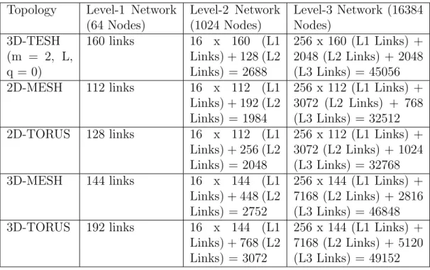
(3.1) Here, equation 3.1 defines required number of inter-connected links for vari-ous levels of networks. The total number of used links for level-1 3D-TESH(2, 1, 0) network is 160, whereas the number of BM for level-1 3D-TESH network is one. This equation has also been generalizes with the required number of links for various networks at table 3.3. On the other hand, table 3.4 shows the example of required number of interconnecting links for various levels of 3D-TESH network, in which cabinet layer the required number of links for 3D-TESH is above 45k. Table 3.4 also shows the link comparison on various networks like- 2D-MESH, 2D-TORUS, 3D-MESH and 3D-TORUS against the 3D-TESH network. The network size for level-1 network has been considered with 64 nodes, level-2 network is having 1024 nodes and level-3 network is consists of 16384 nodes. And from this table we can find that 3D-MESH and 3D-TORUS network require more number of links than the TESH network at the higher levels. This table also shows that 3D-TESH network requires much more number of outgoing links than the two dimensional networks.

(28)

Table 3.3: Generalization of number of links at various levels of 3D-TESH

Topology Level-1 Network Higher Level Network

3D-TESH (Number of X-directional

Links) + (Number of Y-directional Links) + (Number of Z-directional Links)

(Number of BM in current level)×

(Num-ber of inner links in level-1 network) +

∑N

i=2 { (Number of BM at current level,

LN)× (Number of outgoing links at each

higher-level, Li)} [where N ≥ 2]

Table 3.4: Example of required number of links at various levels of networks

Topology Level-1 Network

(64 Nodes) Level-2 Network (1024 Nodes) Level-3 Network (16384 Nodes) 3D-TESH (m = 2, L, q = 0) 160 links 16 x 160 (L1 Links) + 128 (L2 Links) = 2688 256 x 160 (L1 Links) + 2048 (L2 Links) + 2048 (L3 Links) = 45056 2D-MESH 112 links 16 x 112 (L1 Links) + 192 (L2 Links) = 1984 256 x 112 (L1 Links) + 3072 (L2 Links) + 768 (L3 Links) = 32512 2D-TORUS 128 links 16 x 112 (L1 Links) + 256 (L2 Links) = 2048 256 x 112 (L1 Links) + 3072 (L2 Links) + 1024 (L3 Links) = 32768 3D-MESH 144 links 16 x 144 (L1 Links) + 448 (L2 Links) = 2752 256 x 144 (L1 Links) + 7168 (L2 Links) + 2816 (L3 Links) = 46848 3D-TORUS 192 links 16 x 144 (L1 Links) + 768 (L2 Links) = 3072 256 x 144 (L1 Links) + 7168 (L2 Links) + 5120 (L3 Links) = 49152

3.5 Addressing of Nodes

Nodes in a BM are addressed by three digits; the first is the Y-index, then the X-index and finally the Z-index. In general, in a Level-L 3D-TESH, the node address can be represented by:

(29)

AL =      (ayL, axL, azL) if L = 1 (ayL, axL) if Lmax ≥ L ≥ 2

More generally in a Level-L 3D-TESH, the node address is represented

by-A = by-AL AL−1 AL−2 ... ... ... A2 A1

= (a2L, a2L−1) (a2L−2, a2L−3)... ... (a4, a3) (a2, a1, a0)

(3.2)

Here, the Level-1 is defined by node address (a2, a1, a0), where a0 defines

the node address for Z-axis and then followed by the X-axis and then the Y-axis. Level-2 to Level-5 Networks are two dimensional networks, so first digit defines the row index and then the next is the column index. Now

if the address of a node n1 _{included in BM}

1 is represented as n1 = [(s2L,

s2L−1)... ...(s4, s3) (s2, s1, s0)] and the address of a node n2 included in BM2

is represented as n2 _{= [(d}

2L, d2L−1)... ...(d4, d3) (d2, d1, d0)]. The node n1 in

BM1 and n2 in BM2 are connected if the following connections are satisfied

for n2(when m = 2, q = 0)-• Link for BM-[(s2L, s2L−1)... ...(s4, s3) (s2, s1, s0)] to [(s2L, s2L−1)... ...(s4, s3) (s2±1, s1 ± 1, s0± 1 mod 2m)] where 2m_{− 1 > s} 2 > 0, 2m− 1 > s1 > 0, 2m _{> s} 0 ≥ 0, not both s1, s2 ± [(s2L, s2L−1)... ...(s4, s3) (s2, s1, s0)] to [(s2L, s2L−1)... ...(s4, s3) (s2+ 1, s1, s0± 1 mod 2m)] where s2 = 0, 2m > s1, s0 ≥ 0 [(s2L, s2L−1)... ...(s4, s3) (s2, s1, s0)] to [(s2L, s2L−1)... ...(s4, s3) (s2, s1 + 1, s0± 1 mod 2m)] where s1 = 0, 2m > s2, s0 ≥ 0 [(s2L, s2L−1)... ...(s4, s3) (s2, s1, s0)] to [(s2L, s2L−1)... ...(s4, s3) (s2, s1 − 1, s0± 1 mod 2m)] where s1 = 2m− 1, 2m > s2, s0 ≥ 0

(30)

[(s2L, s2L−1)... ...(s4, s3) (s2, s1, s0)] to [(s2L, s2L−1)... ...(s4, s3) (s2−1,

s1, s0± 1 mod 2m)] where s2 = 2m− 1, 2m > s1, s0 ≥ 0

• Link for L2 Vertical- [(s2L, s2L−1)... ...(s4, s3) (0, 0, s0)] to [(s2L, s2L−1)...

...(s4± 1 mod 2m, s3) (0, 0, s0)]

• Link for L2 Horizontal- [(s2L, s2L−1)... ...(s4, s3) (0, 2m − 1, s0)] to

[(s2L, s2L−1)... ...(s4, s3± 1 mod 2m) (0, 2m− 1, s0)]

• Link for L3 Vertical- [(s2L, s2L−1)... ...(s6, s5) ... (2m − 1, 0, s0)] to

[(s2L, s2L−1)... ...(s6± 1 mod 2m, s5) ... (2m− 1, 0, s0)]

• Link for L3 Horizontal- [(s2L, s2L−1)... ...(s4, s3) (2m − 1, 2m− 1, s0)]

to [(s2L, s2L−1)... ...(s6, s5 ± 1 mod 2m) ... (2m− 1, 2m− 1, s0)]

• Link for L4 Vertical- [(s2L, s2L−1)... ...(s8, s7) ... (2, 0, s0)] to [(s2L,

s2L−1)... ...(s8 ± 1 mod 2m, s7) ... (1, 0, s0)]

• Link for L4 Horizontal- [(s2L, s2L−1)... ...(s8, s7) ... (0, 2, s0)] to [(s2L,

s2L−1)... ...(s8, s7± 1 mod 2m) ... (0, 1, s0)]

• Link for L5 Vertical- [(s10, s9)... ...(s4, s3) (2, 3, s0)] to [(s10, s9)...

...(s4, s3) (1, 3, s0)]

• Link for L5 Horizontal- [(s10, s9)... ...(s4, s3) (3, 2, s0)] to [(s10, s9)...

...(s4, s3) (3, 1, s0)]

Similarly, we can define various level of interconnections as above when q = 1 or q = 2 with vertical and horizontal connections. The highest level

of network which can be obtained by a (2m × 2m × 2m) BM is defined by

Lmax = 2m−q+ 1. When m = 2 and q = 0, Lmax = 5; level-5 is the maximum

possible level. In the rest of the paper, we have considered m = 2 and inter-connectivity q = 0; therefore, we focus on the class of 3D-TESH(2, L, 0).

3.6 Routing Algorithm for 3D-TESH

A simple deterministic, dimension-order routing (DOR) algorithm has been considered for 3D-TESH network. DOR routes a packet continuously in each dimension until the distance of that dimension is zero, then forwards to the

(31)

next dimension. Routing of messages for 3D-TESH is performed from top to bottom similar to TESH [5] network. For every message the routing for 3D-TESH network completes at the highest level of network first; after that the packet reaches its highest level sub-destination, routing continues with the sub-network to the next lower level sub-destination. This process is repeated until the packet arrives at its final destination BM and then completes level-1 routing at the destination BM. When a packet is generated at a source node,

the node checks its destination. If the packet ’s destination is the current

BM, the routing is performed with the BM only. If the packet is destined to another BM, the source node sends the packet to the outlet node which connects the BM to the level at which the routing is performed. Let a source

node address is s = (s2L, s2L−1) (s2L−2, s2L−3) ... ... (s4, s3) (s2, s1, s0) and

destination node d = (d2L, d2L−1) (d2L−2, d2L−3) .. ... (d4, d3) (d2, d1, d0)

considering the routing at the Y,X direction for the higher levels and Y, X, Z direction for the level-1 networks. Similarly, routing tag can be defined

as t = (t2L, t2L−1) (t2L−2, t2L−3)... ...(t4, t3) (t2, t1, t0), where ti = di

-si. Algorithm 1 shows the routing algorithm for 3D-TESH network, whereas

algorithm 2 & 3 defines the function outlet x, outlet y, receiving nodex and

receiving nodey.

The function SP routing is used to find the route direction from the source BM towards the destination BM. On the other hand, outlet x and

outlet y are the function to get x coordinate s1 and y coordinate s2 of the

node that link (s, d, l, dα) exists, where level l(2 ≤ l ≤ L), dimension d(d ∈

{V,H}) and direction α(α ∈ {+,-}). Hence vertical and horizontal direction

are represented by V+, V-, H+ and H-. Please find the Appendix A for implemented routing code for 3D-TESH(2, L, 0) network.

(32)

Algorithm 1 Routing Algorithm for 3D-TESH Network Routing 3D-TESH(s2L, s2L−1, s2L−2,……, s1, s0, d2L, d2L−1, d2L−2,……, d1, d0);

tag: t2L, t2L−1, t2L−2,……, t1, t0;

for i = 2L : 3;

routedir = SP routing(s, d,⌊(i − 1)/2 + 1⌋, i);

if (routedir = positive) then ti= ((di- si+ 2m) mod 2m);

else ti= (2m- (di- si+ 2m) mod 2m); endif;

while (ti≠ 0) do

if (i mod 2) = 1, then outlet nodex= outlet x(s, d,⌊(i − 1)/2 + 1⌋, H, routedir);

outlet nodey= outlet y(s, d,⌊(i − 1)/2 + 1⌋, H, routedir);

else outlet nodex= outlet x(s, d,⌊(i − 1)/2 + 1⌋, V, routedir);

outlet nodey= outlet y(s, d,⌊(i − 1)/2 + 1⌋, V, routedir); endif;

BM routing(s2, s1, 0, outlet nodey, outlet nodex, 0);

if (routedir = positive) then send the packet to the next BM; else move the packet to previous BM; endif;

if (ti> 0) then ti= ti- 1; endif;

if (ti< 0) then ti= ti+ 1; endif;

if (i mod 2) = 1, s1= receiving nodex(s, d,⌊(i − 1)/2 + 1⌋, H, routedir);

s2= receiving nodey(s, d,⌊(i − 1)/2 + 1⌋, H, routedir);

else s1= receiving nodex(s, d,⌊(i − 1)/2 + 1⌋, V, routedir);

s2= receiving nodey(s, d,⌊(i − 1)/2 + 1⌋, V, routedir); endif;

endwhile; endfor; BM routing(s2, s1, s0, d2, d1, d0); end BM routing(s2, s1, s0, d2, d1, d0); source: s2, s1, s0; destination: d2, d1, d0;

BM tag: t2, t1, t0= destination address(d2, d1, d0) - source address(s2, s1, s0);

if (t0 > 0 and t0≤ 2m−1) or (t0 < 0 and t0= - (2m- 1)), movedir = positive; endif;

if (t0 > 0 and t0= (2m- 1)) or (t0 < 0 and t0≥ -2m−1), movedir = negative; endif;

if (movedir = positive and t0 > 0) then t0= t0; endif;

if (movedir = positive and t0 < 0) then t0= m + t0; endif;

if (movedir = negative and t0 < 0) then t0 = t0; endif;

if (movedir = negative and t0 > 0) then t0 = -m + t0; endif;

while(t0 ≠ 0) do

if (t0 > 0) then move packet to +z node; t0 = t0 - 1; endif;

if (t0 < 0) then move packet to -z node; t0= t0+ 1; endif;

endwhile; while(t1 ≠ 0) do

if (t1 > 0) then move packet to +x node; t1 = t1- 1; endif;

if (t1 < 0) then move packet to -x node; t1= t1+ 1; endif;

endwhile; while(t2 ≠ 0) do

if (t2 > 0) then move packet to +y node; t2 = t2- 1; endif;

if (t2 < 0) then move packet to -y node; t2= t2+ 1; endif;

endwhile; end

SP routing(s, d, Level, i);

if ((di- si+ 2m) mod 2m) > 2m/2, then routedir = negative;

elseif ((di- si+ 2m) mod 2m) = 2m/2,{

if (Level mod 2) = 0, then

if (i mod 2) = 0, then routedir = positive; else routedir = negative; endif;

else

if (i mod 2) = 0, then routedir = negative; else routedir = positive; endif;}

(33)

Algorithm 2 function definition for 3D-TESH Network

outlet x(s, d, L, V H, rd); //This function is applicable for only 3D-TESH(m, L, 0) if (VH = V and rd = positive) then{

if (L = 2) then outlet nodex= 0; elseif (L = 3) then outlet nodex= 0;

elseif ((L mod 2) = 0) then outlet nodex= 0;

elseif ((L mod 2)≠ 0) then outlet nodex= 2m− 1; else ”Error”; }

if (VH = H and rd = positive) then{

if (L = 2) then outlet nodex= 2m− 1; elseif (L = 3) then outlet nodex= 2m− 1;

elseif ((L mod 2) = 0) then outlet nodex= L - 2;

elseif ((L mod 2)≠ 0) then outlet nodex= L - 3; else ”Error”;}

if (VH = V and rd = negative) then{

if (L = 2) then outlet nodex= 0; elseif (L = 3) then outlet nodex= 0;

elseif ((L mod 2) = 0) then outlet nodex= 0;

elseif ((L mod 2)≠ 0) then outlet nodex= 2m− 1; else ”Error”; }

if (VH = H and rd = negative) then{

if (L = 2) then outlet nodex= 2m− 1; elseif (L = 3) then outlet nodex= 2m− 1;

elseif ((L mod 2) = 0) then outlet nodex= L - 3;

elseif ((L mod 2)≠ 0) then outlet nodex= L - 4; else ”Error”;}

end

outlet y(s, d, L, V H, rd); //This function is applicable for only 3D-TESH(m, L, 0) if (VH = V and rd = positive) then{

if (L = 2) then outlet nodey= 0; elseif (L = 3) then outlet nodey= 2m− 1;

elseif ((L mod 2) = 0) then outlet nodey= L-2;

elseif ((L mod 2)≠ 0) then outlet nodey= L - 3; else ”Error”;}

elseif ((L mod 2) = 0) then outlet nodey= 0;

elseif ((L mod 2)≠ 0) then outlet nodey= 2m− 1; else ”Error”; }

elseif ((L mod 2) = 0) then outlet nodey= L - 3;

elseif ((L mod 2)≠ 0) then outlet nodey= L - 4; else ”Error”;}

if (VH = H and rd = negative) then{ if (L = 2) then outlet nodey= 0;

elseif (L = 3) then outlet nodey= 2m− 1;

elseif ((L mod 2) = 0) then outlet nodey= 0;

elseif ((L mod 2)≠ 0) then outlet nodey= 2m− 1; else ”Error”; }

end

receiving nodex(s, d, L, V H, rd); //This function is applicable for only 3D-TESH(m, L, 0)

if (VH = V and rd = positive) then{

if (L = 2) then receiving nodex = 0; elseif (L = 3) then receiving nodex = 0; elseif ((L mod 2) = 0) then receiving nodex = 0;

elseif ((L mod 2)≠ 0) then receiving nodex = 2m_{− 1; else ”Error”; }}

if (L = 2) then receiving nodex = 2m− 1; elseif (L = 3) then receiving nodex = 2m− 1; elseif ((L mod 2) = 0) then receiving nodex = L - 3; elseif ((L mod 2)≠ 0) then receiving nodex = L - 4; else ”Error”;}

if (L = 2) then receiving nodex = 0; elseif (L = 3) then receiving nodex = 0;

elseif ((L mod 2) = 0) then receiving nodex = 0; elseif ((L mod 2)≠ 0) then receiving nodex = 2m_{− 1; else ”Error”; }}

if (L = 2) then return receiving nodex = 2m_{− 1; elseif (L = 3) then return receiving nodex =}

2m_{− 1;}

elseif ((L mod 2) = 0) then receiving nodex = L - 2; elseif ((L mod 2)≠ 0) then receiving nodex = L - 3; else ”Error”;}

(34)

Algorithm 3 function definition for 3D-TESH Network

receiving nodey(s, d, L, V H, rd); //THIS function is applicable for only 3D-TESH(m, L, 0)

if (VH = V and rd = positive) then{

if (L = 2) then return receiving nodey = 0; elseif (L = 3) then return receiving nodey = 2m_{− 1;}

elseif ((L mod 2) = 0) then receiving nodey = L - 3; elseif ((L mod 2)≠ 0) then receiving nodey = L - 4; else ”Error”;}

if (L = 2) then receiving nodey = 0; elseif (L = 3) then receiving nodey = 2m_{− 1;}

elseif ((L mod 2) = 0) then receiving nodey = 0; elseif ((L mod 2)≠ 0) then receiving nodey = 2m− 1; else ”Error”; }

elseif ((L mod 2) = 0) then receiving nodey = L - 2; elseif ((L mod 2)≠ 0) then receiving nodey = L - 3; else ”Error”;}

elseif ((L mod 2) = 0) then receiving nodey = 0; elseif ((L mod 2)≠ 0) then receiving nodey = 2m_{− 1; else ”Error”; }}

end

To understand the routing path for TESH network using the 3D-TESH DOR routing algorithm we have considered figure 3.4 where the source node is (1,2),(1,2),(1,2,0) and the destination node is (2,1),(2,1),(2,1,0). At first routing will be done at Level-3 network, the source node will send the packet to the outlet node (1,2),(1,2),(3,0,0) of Level-3 network and will reach Level-3(2,2) from Level-3(1,2) network. Similarly, it will reach Level-3(2,1) network. Then, 2(1,2) routing will be started and will reach Level-2(2,1) network. After that in Level-1 network packet will reach the destina-tion Node(2,1,0) from the destinadestina-tion BM Node(0,3,0).

3.7 Summary

In recent, a large number of interconnection networks have been proposed to minimize the cost and to maximize the performance. Hierarchical inter-connection networks are ahead of others. In this chapter, we have described about the architecture of 3D-TESH network. The addressing, message rout-ing of 3D-TESH and the routrout-ing algorithm of 3D-TESH were described in details. Higher level of 3D-TESH is maintained by the immediate lower level of subnetworks. Higher level interconnection of 3D-TESH is also described in this chaptor.

(35)

Figure 3.4: Routing Path for 3D-TESH Network

(36)

Chapter 4 Static Network Performance

Evaluation

4.1 Introduction

The topology of interconnection network aﬀects the performance metrics. Performance metrics can be used to evaluate and compare diﬀerent network topologies. It is being expected from the interconnection network with low cost, low degree, low congestion, high connectivity, and high fault tolerance than the other networks. In this chapter, we will compare the static net-work performance like- the node degree, diameter, average distance, cost performance, the bisection bandwidth and arc connectivity of various inter-connection networks against the 3D-TESH network.

4.2 Comparison of Static Performance of

Var-ious Networks

4.2.1 Node Degree

The node degree is defined as the maximum number of physical outgoing links from a node. Since each node of 3D-TESH network has maximum six outgoing links, the degree of 3D-TESH is 6. Constant node degree networks are easy to expand and the network interface cost remains unchanged with increasing network size. The I/O interface cost of a particular node is pro-portional to its degree. Table 4.1 shows the node degree for the various

(37)

networks.

Table 4.1: Node Degree of Various Networks

Parameter 2D-Mesh 2D-Torus TESH Network 3D-TESH

Node Degree 4 4 4 6

4.2.2 Diameter Performance

A node must follow a communication path to transmit data to other node which are not directly connected. Increase of path length increases the com-munication delay. Shortest path is desirable. The diameter of a network is the maximum inter-node distance i.e., the maximum number of links that must be traversed to send a message to any node along the shortest path. Diameter is the maximum distance between all distinct pairs of nodes along the shortest path. Network with small diameter is preferable. If the diameter is preferable it will take less time to route a packet. Diameter is a common approach to compare the static network performance of a network topology. It has been shown from the figure 4.1 that the 3D-TESH has the diameter less than 2D-MESH, 2D-TORUS, TESH networks for any hierarchical level of network.

Diameter for 3D-TESH can also be evaluated using the below equation-Diameter = maximum value to make the Z-directional routing + maximum value to move to the highest level of outgoing node + then make the highest level routing + maximum value to go to the next level routing out going node + make the next level routing + this loop will continue as it moves to the level-2 + from level-2 incoming node to the destination node.

For the 3D-TESH network, an upper bound for the diameter is given

by-Diameter = max(Dz+ Ds+ ( L

∑

i=2

(Dsi+ Di)) + Dd) (4.1)

(38)

2 8 2 9 2 10 2 11 2 12 2 13 2 14 2 15 2 16 2 17 2 18 2 19 2 20 2 21 2 3 2 4 2 5 2 6 2 7 2 8 2 9 2 10 2 11 D i a m e t e r Number of Nodes 2DM 2DT 3DM 3DT 5DT TESH(2, L, 0) 3DTESH(2, L, 0) TTN(2, L, 0) STTN(2, L, 0) Figure 4.1: Diameter Performance for Various Networks

highest level of outgoing node. Dsi is the value to go to the next level of

routing and Di is the corresponding level of routing. Dd is the value from

level-2 to destination node. Table 4.2 shows the calculated formulation for 3D-TESH

network-4.2.3

Average Distance

It is not always preferable to compare the network performance against only the diameter because a node has to communicate with others; hence on an average, shorter path than the lower diameter is being expected. The average distance is the mean distance between all distinct pairs of nodes in a net-work. Small average distance is preferable which allows small communication latency. Figure 4.2 shows the average distance for various networks.

4.2.4 Cost Performance

Inter-node distance, message traﬃc density, and fault- tolerance are depen-dent on the diameter and the node degree. Hence the product of node degree and diameter is useful for measuring the relationship between cost and perfor-mance of a multiprocessor system. Figure 4.3 shows the total cost of TESH

(39)

Table 4.2: Calculated Formulation of Diameter for 3D-TESH Network.

Parameter Result

of Dz

Result

of Ds

Result for Dsi and Di Result

for Dd Diameter of the corre- spond-ing level Level-1 network 2 6 Dsi = 0, Di = 0 0 8

Level-2 network 2 6 for i = 2; Dsi=0, Di=7 6 21

Level-3 network 2 6 for i = 2; Dsi=0, Di=7

for i = 3; Dsi=0, Di=7

6 34

and 3D-TESH with respect to other networks. TESH shows lower cost than 3D-TESH, as the node degree of 3D-TESH is greater than TESH.

4.2.5 Bisection Bandwidth

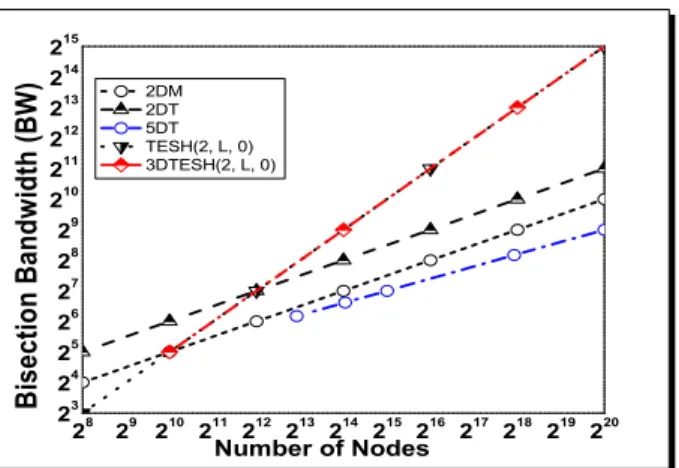
The Bisection Bandwidth (BW) of a network is defined as the minimum number of links that must be removed to partition the network into two equal halves. Small bisection bandwidth implies low bandwidth between the two halves and it can slow down the final merging phase. A large bisection bandwidth is undesirable for the VLSI design of the interconnection network, since it implies a lot if extra chip wires. Figure 4.4 shows the bisection bandwidth of the various networks.

The bisection bandwidth for 3D-TESH(m, L, q) is given by:

BW3D−T ESH(m,L,q) = 2m× 22m(L−1)−1× 2m+1

= 2m(2L−3)+1 × 2m [ L ≥ 2 ] (4.2)

4.2.6 Arc Connectivity

Arc Connectivity measures the robustness of a network. It is a measure of the multiplicity of paths between the processors. Arc connectivity is the minimum number of links that must be removed in order to break the network

(40)

2 8 2 9 2 10 2 11 2 12 2 13 2 14 2 15 2 16 2 17 2 18 2 19 2 20 2 21 2 22 2 2 2 3 2 4 2 5 2 6 2 7 2 8 2 9 A v e r a g e D i s t a n c e Number of Nodes 2DM 2DT 3DM 3DT 5DT T ESH(2, L, 0) T T N(2, L, 0) 3DT ESH(2, L, 0) Figure 4.2: Average Distance for Various Networks

T ESH(2, L, 0) 3DT ESH(2, L, 0) T T N(2, L, 0)

Figure 4.3: Cost Performance for Various Networks

(41)

2 8 2 9 2 10 2 11 2 12 2 13 2 14 2 15 2 16 2 17 2 18 2 19 2 20 2 3 2 4 2 5 2 6 2 7 2 8 2 9 2 10 2 11 2 12 2 13 2 14 2 15 B i s e c t i o n B a n d w i d t h ( B W ) Number of Nodes 2DM 2DT 5DT TESH(2, L, 0) 3DTESH(2, L, 0) Figure 4.4: Bisection Bandwidth for Various Networks

into two disjoint parts. High arc connectivity improves performance during normal operation by avoiding link congestion and improved fault tolerance. A network is maximally fault tolerant if its connectivity is equal to the degree of that network. Table 4.3 shows arc connectivity of various networks.

Table 4.3: Arc Connectivity for Various Networks

Parameter 2D-Mesh 2D-Torus TESH Network 3D-TESH

Node Degree 4 4 4 6

Arc Connectivity 2 4 2 4

4.3 Summary

The above six parameters are normally used to determine the static perfor-mance of a network. Diameter and average distance is the most important consideration for the evaluation of static network performance. Because lower diameter of a network takes shorter time to send a message from source node to destination node. Similarly if the average distance is short, the static net-work performance would be improved. Cost of a netnet-work is totally belongs to node degree. As the node degree of 3D-TESH is high, the cost performance of 3D-TESH is greater than the two dimensional TESH network.

(42)

Chapter 5 Dynamic Communication

Performance Evaluation

5.1 Introduction

Bad performance of the communicational network will severely limit the speed and eﬃciency of the entire MPC system. The dynamic communi-cation performance (DCP) of an interconnection network is characterized by latency and throughput. Message latency is the time required for a packet to traverse the network from source to destination. Therefore, it refers to the time elapsed from the instant when the last flit of the message is received at the destination. Latency can be described as:

T = Th+ L/b, Ts= L/b (5.1)

Here, the head latency Th, is the time required for the head of the message

to traverse the network. The serialization latency Ts, is the time required

for a packet of length L to cross a channel with bandwidth b. Network throughput is the rate at which packets are delivered by the network for a particular traﬃc pattern. It refers to the maximum amount of information delivered per unit of time through the network.

5.2 Estimation of Power Consumption

Power dissipation is a major concern for the next generation of supercom-puters. The k-computer with Tofu interconnect requires about 9.89MW of

(43)

electrical power to run the complete system [4]. The power model for 3D-TESH can be defined by 2-ways; one is on-chip power model and other is the oﬀ-chip power model.

The on-chip power model is based on the Orion energy model [18] using 65nm fabrication process, considering the static and dynamic power dissipa-tion within the routers and in the inter-router interconnects. We have used the GARNET on-chip network model [19] along with the Orion energy model. Inside the GARNET simulator, router informations are collected considering the number of reads, writes to router buﬀers, the activity at the local & global arbiters and finally the total number of crossbar traversals. The total link power is also measured according to Orion link power model. Networks total energy consumption is equal to the sum of energy consumption of all routers and links. The equation 5.2 shows the summation of energy consumption inside a router. The energy of each component depends on the dynamic and

leakage energy. ”The dynamic energy is defined by E = 0.5αCV2, here α

is the switching activity, C is the capacitance and V is the supply voltage” [19]. The capacitance depends on various physical (transistor width, wire length, etc.) and architectural (number of ports, flit size, buﬀer size, etc.) parameters. GARNET transfers the pre-component activity to Orion. On the other hand, total leakage power consumed in the network is the sum of leakage power of router buﬀers, crossbar, arbiters and links.

Erouter = Ebuf f er write+ Ebuf f er read + Evc arb+ Esw arb+ Exb [19] (5.2)

Considering the clock frequency is 1GHz, supply voltage 1.0V, using 128bits message size and uniform traﬃc pattern; table 5.1 shows the sim-ulation condition for level-1 network and table 5.2 shows the power analysis for 3D-TESH(2,1,0) level-1 network with 2mm link length and 1 virtual chan-nel. Figure 5.1 shows the dynamic and static power dissipation for links with 1 virtual channel. Similarly, figure 5.2 shows the power dissipation for to-tal router power for various networks; where 3D-Torus networks shows the worst.

Now, considering the oﬀ-chip network for 3D-TESH we have assumed electrical interconnect with 4Gb/s of link bandwidth. The power model for oﬀ-chip electrical interconnect [20] is based upon the figure 5.3, which shows board-level electrical interconnects and table 5.3 shows the board trace pa-rameters and corresponding SPICE papa-rameters. This electrical power model

(44)

Table 5.1: Simulation condition for level-1 3D-TESH network

Parameter Value Units

Fabrication process 65nm

-number of nodes 64 nodes

-Link length 2 [mm]

Operating frequency 1× 109 _Hz

Transistor type NVT

-Supply voltage 1 V

Traﬃc pattern uniform traﬃc

-Message injection rate 0.01 flits/cycle/node

Message size 128 bits

Simulation cycle 20000

-Table 5.2: Power estimation for various networks(2mm link length, 1 virtual channel & 64 nodes)

Topology Link

Dy-namic Power(W) Link static Power(W) Router dynamic power(W) Router static power(W) Clock Power (W) Router total Power(W) 3D-TORUS 0.116735 0.675740 0.476532 1.502490 3.067085 5.046107 3D-MESH 0.134247 0.574379 0.451448 1.156960 2.492006 4.100415 3D-TESH 0.128555 0.608166 0.457665 1.268284 2.683699 4.409648 2DM 2DT 3DM 3DT 3DTESH 0.00 0.15 0.30 0.45 0.60 0.75 0.90 T o t a l L i n k P o w e r ( W ) Various Topologies Link Static Power(W )

Link Dynamic Power(W )

Figure 5.1: Link Power Analysis for Various Networks

(45)

2DM 2DT 3DM 3DT 3DTESH 0 1 2 3 4 5 6 T o t a l R o u t e r P o w e r ( W ) Various Topologies Clock Power(W )

Router Static Power(W ) Router Dynamic Power(W )

Figure 5.2: Router Power Analysis for Various Networks

considers the power dissipation at the termination resistors and depends on attenuation and noise characteristics of interconnects.

Figure 5.3: Schematic showing board-level electrical interconnects. This fig-ure is obtained from reference [20]

The total power has been obtained from this power model [20] is the sum

of the power consumed in the two termination resistances, where IO is the

required current for one way signaling and Z0 is the impedance. Thus total

power consumption has been defined

(46)

Table 5.3: Board trace parameters and the corresponding SPICE parameters used for dielectric and skin eﬀect. This table is obtained from reference [20].

Parameters Value L 302 [nH/m] C 148 [pF/m] Z0 45 [Ω] R0 4.71 [Ω/m] Rs 1.313× 103 [Ω/m √ Hz] G0 0 Gd 9.929× 10−12 [Ω/mHz]

Figure 5.4 shows the power comparison for oﬀ-chip interconnect of electri-cal and optielectri-cal interconnects with various wire length. This figure explains the power requirement for oﬀ-chip optical interconnect is higher than the electrical interconnect up to a curtain level. But with the increase of the interconnection link length, the power consumption for the electrical inter-connect has been increased much more than the optical interinter-connect. This figure is also been highlighted for electrical interconnect at length 100mm and 1m, which has been used for this research paper.

Now, using the above oﬀ-chip interconnect model we can also simulate the total required power for various levels of 3D-TESH network. To find the total required power at the level-2 3D-TESH network, we have assumed

the oﬀ-chip wire length is 100mm, VN F = 8.8mV , 1 virtual channel and

similarly, to find the total required power at the level-3 3D-TESH network,

we have assumed the oﬀ-chip wire length is 1m, VN F = 8.8mV & 1 virtual

channel. Equation 5.4 shows the definition to calculate the required power at various level of 3D-TESH network, table 5.4 shows the parameter that have been used for calculating the power consumption for higher-level networks and figure 5.5 shows the total power comparison of various levels of network, which explains that 3D-torus network will require much more power than 3D-TESH network with the increase of the network size due to the increased number of outgoing links (section 3.4) at various levels.

(47)

Figure 5.4: Power comparison for oﬀ-chip interconnect. This graph is ob-tained from reference [20]

Total power required for LN network = (Number of BM in current level,

LN)× (power required for L1 network) + N

∑

i=2

{(Total number of outgoing

links from all BM at higher-level, Li) × (power required for each Li link)}

[where N≥ 2 ]

(5.4)

5.3 Definition of Various Traﬃc Patterns

Network load has a very effective influence on performance. In general, for a given distribution of destinations, the average message latency of a VCT switched network is more heavily affected by the network load than by any design parameter, provided that a reasonable choice is made for those pa-rameters. Even throughput is also heavily affected by the traffic patterns,

(48)

Table 5.4: Parameter used for power analysis of various levels of networks

Network Size Links

length

Link band-width

Vgaussian VN F Power

con-sumption (per link) Level-2 Network (1024 Nodes) 100mm 4 Gb/s 5mV 8.8mV 0.0032w Level-3 Network (16384 Nodes) 1m 4 Gb/s 5mV 8.8mV 0.0135w 2 0

2.0E3 4.0E3 6.0E3 8.0E3 1.0E4 1.2E4 1.4E4 1.6E4 200.0 400.0 600.0 800.0 1.0k 1.2k 1.4k T o t a l P o w e r ( W ) Number of Nodes 2DM 2DT 3DM 3DT 3DT ESH(2, L, 0)

JAIST Repository: A new Interconnection Network that achieves High Performance for Many-Core Processors