Convergence of an Integral Equation Method to convective Heat Transfer

(1)

14

Convergence of

an

Integral

Equation

Method

to Convective

Heat Transfer

大西和榮

K. Onishi

Applied Mathematics Department

Fukuoka University

Jonan-ku, Fukuoka 814-01 (Japan)

Contents

1. Introduction

2. Integral Equation of the Second Kind

3. Solution of the Integral Equation 4. Galerkin Approximations

5. Conclusions References Abstract.

A boundary-domain (or hybrid) integral equation method is applied to the approximate solution of

transient convection dominated conduction problems in three dimensions. The domain of interest has non-smooth surface of the Wendland type. Given field velocity is assumed to be non-uniform.

Neumann boundary condition is imposed to the problem. Under some conditions which are not much

restrictivein practical applications in engineering, the integral equationisprovedtobe uniquely solvable in the Banachspace ofcontinuous functions onthe enclosure of the domain with the supremumnorm, _It _is

shown as a direct consequence of the Krasnosel’skii’s result that the computational scheme by the

Galerkinmethod is inversely stable and approximate solutions convergeuniformlyto the exact solution.

数理解析研究所講究録第 691 巻 1989 年 14-26

(2)

15

1. Introduction

Aheat transfer problem to be considered in this paper is loosely stated

as

follows: Given

the flow velocity $v(x)=(v], v_{2} ,v_{3})$ in

a

domain $\Omega$ in three dimensions with rectangular

coordinates

such that the incompressibility condition:

a

$v_{j}$

$=$ $0$ in $\Omega$ , $t>0$ (1)

$\partial x_{j}$

is satisfied, find unknown temperature $u(x,t)$ which satisfies the transientheat convection

conduction

equation: $\partial u$ $\partial u$ – $+v_{j}-$ $=$ $h\Delta u$ in $\Omega$ , $t>0$ (2) $\partial t$ $\partial x_{j}$

subject to the boundary and initial conditions:

$q$

$:=-\lambda\underline{\partial u}$

$+v_{j}n_{j}u$ $=q$

on

$\Gamma=$

a

$\Omega$

.

$t>0$ (3)

$\partial n$ and

$u(x, 0)$ $=$ $u^{0}(x)$ in $\Omega$ (4)

for given total flux $q^{\wedge}$

on

the boundary and given initial temperature distribution $u0(x)$

with given constant heat conductivity $\lambda>0$ and the exterior normal $n=(n_{1}, n_{2}, n_{3})$ to

the boundary F. The proper setting of the problem is presented in the next section. We shall consider the

case

that the boundary $\Gamma$ is

a

non-smooth surface of

some

general kind and correspondingly

we

assume

that the given total flux is not bounded

on

the

boundary. The solution will be found in the space of continuous functions

on

the closure

of the domain.

Transient heat conduction problem with Neumann boundary condition

on

non-smooth

surface

was

considered by Costabel et al. [1987] and Onishi[1987]. They showed the unique existence of the solution of corresponding Volterra-Fredholm integral equation of the second kind and presented the uniform convergence of Galerkin approximate

solu-tions.

The present paper is the extension of those previous two

papers

by including the

convection effectto the heat conduction problem. Owing to the presence of the convection

(3)

16

Aboundary-domain integral equation approach for the Neumann problem of steady

con-vection-diffusion problem

was

considered by Onishi[1987], in which the existence of the

continuous solution is proved at all Peclet numbers.

2. Integral Equation of the Second Kind

We shall derive

an

integral equation corresponding to the initial-boundary value problems

(1)$-(4)$

.

To this end,

we

start with the specification of the domain in question. Let $\Omega$be

a

simply connected and bounded opendomain in $R3$

.

The boundary$\Gamma$ is assumed to be

a

piecewise Ljapunow surface. This

means

that the surface is locally Hoelder continuous with the index $1+\kappa(0<K\leq 1)$

.

We denote the set of non-smooth points

on

the surface

by $\gamma$. It forms edges and

corners.

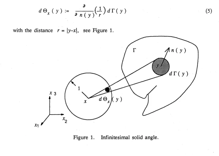
Let $d\Gamma(y)$ be

an

infinitesimal surface

area

at the point $y\in\Gamma-\gamma$

.

The infinitesimal solid

angle at $x(\in R3)$ subtending the

area

$d\Gamma(y)$ is given by the expression:

$d\Theta_{x}(y)$ $;=$ $\frac{3}{\partial n(y)}(\frac{1}{r})d\Gamma(y)$ (5)

with the distance $r=$

I

$y-x|$,

see

Figure 1.

Figure 1. Infinitesimal solid angle.

(4)

$X \in sup_{R^{3}}\int_{\Gamma}|d\Theta_{x}(y)$

{

$=$;

$A$ $<$ $+\infty$ (6)

with

some

constant$A$

.

The solid angle at $x$ subtending to the whole geometry $\Gamma$ is given

by the expression:

$\Theta(x)$ $;= \int d\Theta_{x}(y)=\{\begin{array}{l}4\pi(x\in\Omega^{o})0(x\in\Omega^{ext})\end{array}$ (7)

$y\in\Gamma$

We

assume

moreover

that the boundary $\Gamma$ satisfies the inequality:

$\lim$ _$su^{p}$

$W_{8}(x)=$; $\omega<$ 1 (8)

$8arrow 0$ $x\in\Gamma$

with

some

constant to, in which

$W_{8}(x)$ $;= \frac{1}{4\pi}\{ \int|d\Theta_{X}(y)|+|4\pi-\Theta(x)|\}$ (9)

$0<|y-\chi|\leq 8$

The piecewise Ljapunow surface satisfying the property (8) is called quasi-Wendland

surface.

We notice that the constant $4\pi$ in (9) is replaced by $2\pi$ for the integral equation

defined only

on

the boundary

as

discussed in Wendland[1968]. The assumption (8) im-plies the inequality $4\pi(1-\omega)\leq\Theta(x)$.

Let the Neumann data $q^{\wedge}( t)$ be in the space of$pth$

-power

summable functions $Lp(\Gamma)$

with$p>2$

.

We

assume

that

$\Vert\hat{q}$ (. t) $\Vert_{p}$

$;= \{\int_{\Gamma}|\hat{q}(X, t)|^{p}d\Gamma\}1/p\leq$ $M_{1}$ (10)

uniformly for all $t\in[o,\eta$ with

some

constant $M_{1}$. The boundary condition (3) is under-stood in the

sense

of the boundary flow;

see

Onishi[1986].

As in Costabel et al.[1986],

we can see

that the solution $u(x,t)$ of the initial-boundary

(5)

18

$u$ $( x, t)=- \lambda\int_{0^{d}}^{t}\tau\int_{\Gamma}u(y, \tau)h^{*}(y, \tau:X, t)d\Theta_{x}(y)$

$+ \int_{0^{d}}^{t}\tau\int_{\Omega}u$ _{$(y , \tau)v_{j}(y, \tau)\frac{su^{*}}{sx}(yj , \tau :} _{X, t)d\Omega$} (11)

$- \int^{t}d\tau\int\wedge q(y, \tau)u^{*}$

( $y,$ $\tau:X$ , t) $d \Gamma+\int^{t}d\tau\int u^{o}(y)u^{*}$( _$y,$ $0$ ; $X$ , t) $d\Omega(y)$

,

$0$ $\Gamma$ _$0$ $\Omega$

where $u^{*}$ is the fundamental solution to the heat operator, i.e.,

$\frac{au^{*}}{\partial T}+\lambda\Delta_{y}u^{*}=-8(y-x)8(t-\tau)$

, (12)

$u^{*}= \{(\frac{1}{2\sqrt{}\overline{\pi\lambda(t-\mathcal{T})}}\int\exp 0[-\frac{r2}{4\lambda(t-\mathcal{T})}]$ _{$(t(t>\tau)<\tau)$} (13)

and

$h^{*}( \mathcal{Y}, \tau:x, t)=\frac{r^{3}}{2h(t-\tau)}u^{*}(\mathcal{Y}, \tau:x, t)$ ₍₁₄₎

We notice that all integrals involved in (11)

are

weakly singular inthe

sense

thatthey

are

absolutely convergent. This nice property is due to the assumption that the surface is piecewise Ljapunow. We shall show here the weaksingularity only forthe first integral

on

the right hand side of (11). In fact,

on

each subsurface $\Gamma_{i}$

, the integral is written in the

form:

$\int^{t}d\tau\int u(y, \tau)h^{*}(y, \tau:x, t)d\Theta_{x}(y)$

$0$ $r_{i}$

$= \int^{t}d\tau\int u(y, \tau)\underline{su}(y, \tau:X, t)d\Gamma$

$0$ _{$r_{i}$}

a

$n$

(6)

19

$*$

a

$u$ $-(y, \tau:x, t)$

a

$n$ $=( \frac{1}{2\sqrt{}\overline{\pi h(t-\tau)}}\int[\frac{-r}{2\lambda(t-\tau)}]\exp[\frac{-r2}{4\lambda(t-\tau)}]\frac{y.-X}{r}n_{j}(y)$

Since $\Gamma i$ is

a

Ljapunow surface, it follows that

$|\underline{y.-X\cdot}n.(y)|=|\cos v|$ $\leq L(\Gamma)|y-x|^{K}$

$r$ $J$

for the angle $v$ between two vectors _$y-x$ and $n(y)$ with the constant$L$. Using the inequality

$\xi^{S}e^{-g}\leq s^{s}e^{-s}(s>0)$ _,

we

can see

that $*$

$| \frac{\partial u}{n}\partial$ ( $y,$ $\tau:x$ , t)

$|$ _{$\leq\frac{c_{1}}{(t-\tau)}\mu\frac{L(\Gamma)}{r^{4-2\mu-K}}$}

for all $\mu<1$ with

some

constant $G1$. Choose $\mu$

so

that $4-2\mu-\kappa<2$

.

This implies that

$1-\kappa/2<\mu<1$ and the integral is absolutely convergent.

As regard to the continuity of the second and third integrals in (11),

we

have Lemma 1.

(1).

_If

$q^{\wedge}is$ in $C(Lp(\Gamma):[o,\eta)$ with $p>2$, then the single-layer heat potential:

$\int^{t}d\tau\int\wedge q(y, \tau)u^{*}$

( $y,$ $\tau:x$ , t) $d\Gamma$ $\in C(R3\cross[0, \infty))$

$0$ $\Gamma$

(2).

_If

$\mathcal{V}j(\chi)$ is continuous in the closure

of

$\Omega$, then the volume heat potential: $*$

$\int_{0^{d}}^{t}\tau\int_{\Omega}u(y, \tau)v_{j}(y, \tau)\frac{\partial u}{\partial\chi}$ ( $y1$ ,

$\tau$ : $x$ , t) $d\Omega\in C$

$( R3\cross[0, \infty))$

One of the advantages of the integral equation approach is that

one can

treat the

continu-ous

function

even

if the Neumann data $q^{\wedge}$

are

discontinuous

on

the boundary.

Take

a

point $x\in\Gamma-\gamma$

.

We know the jump relation for the double-layer heat potential in the form:

(7)

20

$\lim$ $\int^{t}d\tau\int u(y, \tau)h^{*}(y, \tau:z, t)d\Theta_{Z}(y)$ $Zarrow X$ $0$ $\Gamma$

$z\in\Omega^{O}$

(15)

$=- \frac{1}{2\lambda}u(x, t)+\int_{0^{d}}^{t}\tau\int_{\Gamma}u(y, \tau)h^{*}(y, \tau:x, t)d\Theta_{x}(y)$

The integral appearing

on

the right hand side is defined

so

far only at points $x$

on

the

smooth boundary. However, it

can

be completed to be

a

continuous function

on

the whole boundary F. The value at the point $\xi\in\gamma$ is given from the relation:

$\lim$ $\int^{t}d^{r}r\int u(y, \tau)h^{*}$( _$y$ , $\tau$ : $x$ , t)

$d\Theta_{X}(y)$

$Xarrow\xi$ $0$ $\Gamma$

$\xi\in\Gamma-\gamma$ (16)

$=- \frac{1}{2\lambda}(1-\frac{\Theta(\xi)}{2\pi})u$ ( $\xi$ , t) $+ \int_{0^{d}}^{t}\tau\int_{\Gamma}u(y, \tau)h^{*}$( _$y,$ $\tau$ : $\xi$ , t)

$d\Theta_{\xi}(y)$

By combining (11), (15), and (16),

we see

thatthe unknown$u(x,t)$ at all $x\in\Omega\cup\Gamma$ is given by the solution of the following integral equation:

$u(X, t)= \frac{1}{2}(2-\frac{\Theta(x)}{2\pi})u$ ( $X$ , t)

$- \lambda\int_{0^{d}}^{t}\uparrow\int_{\Gamma}u(y, \tau)h^{*}(y, \tau:x, t)d\Theta_{x}(y)$

$+ \int_{0\Omega}d^{t}\tau\int u(y, \tau)v_{j}(y, \tau)\frac{\partial u^{*}}{X}$ (

$y3j$

$\tau:x$ , t) $d\Omega$

(17)

$- \int^{t}d\tau\int\wedge q(y, \tau)u^{*}(y, \tau:X, t)d\Gamma+\int^{t}d\tau\int u^{o}(y)u^{*}(y, 0 : x, t)d\Omega(y)$

$0$ $\Gamma$ $0$ $\Omega$

This equation is regarded

as a

Volterra-Fredholm integral equation of the second kind.

The equation involves not only integrals

on

the boundary but integrals defined

on

the

(8)

3. Solution of the Integral Equation

We shall consider the existence of the solution of integral equation (17) in the Banach

space

of continuous functions $C$$( \overline{\Omega}\cross[0, T])$ equipped withthe supremum

norm.

To

this end

we

shall introduce integral operators according to the following definitions:

$Qu$ ( $x$ , t) $:= \frac{1}{2}(2-\frac{\Theta(x)}{2\pi})u(x, t)$

(18)

$-h \int^{t}d\tau\int$ _{$u(y, \tau)h^{*}(y, \tau:x, t)d\Theta_{x}(y)$}

$00<|y-x|\leq 8$

$y\in\Gamma$

Vu $(x, t)$ $;=-h \int^{t}d\tau\int u(y, \tau)h^{*}$₍

$y,$ $\tau:x$ , t) $d\Theta_{x}(y)$ (19)

$08<|y-x|$

$y\in\Gamma$

$*$

$Wu(x, t):= \int_{0^{d}}^{t}\tau\int_{\Omega}u(y, \tau)v_{j}(y, \tau)\frac{au}{X}$ ( $y\partial j$

$\tau$ : $x$ , t) $d\Omega$ (20)

and

$g$ ( $X$ , t) $;=- \int^{t}d\tau\int\wedge q(y, \tau)u^{*}(y, \tau:x, t)d\Gamma$

$0$ $\Gamma$

(21)

$+ \int^{t}d\tau\int u^{\circ}(y)u^{*}(y, 0 ; x, t)d\Omega(y)$

$0$ $\Omega$

Here, $g(x,t)$ is regarded

as

known continuous function. The integral equation (17) is

now

written in the form:

(9)

22

Lemma 2.

_If

$\Gamma$ is the quasi-Wendland surface, then it holds that

(i). $Q$ is

a

contraction in $C$$( \overline{\Omega}\cross[0, T])$

for

some

sufficiently small 8,

(ii). $V$ is completely continuous in $C(\overline{\Omega}\cross[0, T])$ with that 8

as

above, and

(iii). $W$ is completely continuous in $C$$( \overline{\Omega}x[0, T])$

Proof.

For the proof of (ii) and (iii),

see

Onishi[1987]. We shall show

an

outline of the

proof of (i) here. First for $x\in\Omega$,

we see

that

$Q_{\mathcal{U}}( \chi, t)=-\lambda\int^{t}d\tau\int u(\mathcal{Y}, \tau)h^{*}(\mathcal{Y}, \tau:x, t)d\Theta_{x}(\mathcal{Y})$

$00<|y-x|\leq 8$ It follows that

$|Qu(X, t)|$

$\leq\lambda\int|d\Theta_{X}(y)|\int_{0}\frac{{}^{t}r^{3}}{2\lambda(t-\tau)}0<|y-x|\leq 8(\frac{1}{2\sqrt{}\overline{\pi h(t-\tau)}}\int\exp[-\frac{r2}{4h(t-\uparrow)}]d\tau\Vert u\Vert$

with $\Vert u||$ $:=$ $\max|u$ $(x , t)|$ $\overline{\Omega}\cross[0, T]$

To evaluate integrals

we use

the variable transformation:

$\taurightarrow 0=\frac{\gamma 2}{2\sqrt h(t-\tau)}$ which implies

$0^{2}= \frac{r2}{4h(t-\uparrow)}$ $t- \tau=\frac{r2}{4\lambda 0^{2}}$ $d \tau=\frac{r2}{2\lambda 0^{3}}do$

Then

we

see

$|Qu(X, t)| \leq h\int|d\Theta_{x_{|\leq 8}^{(y)1\int_{\frac{r\infty 20}{2\sqrt{\lambda t}}}}}0<|y-X2_{\Gamma}(\frac{o}{\sqrt{\pi}r})^{3}e^{-0}\frac{2r2}{2ho^{3}}do$

(10)

23

$\leq\frac{1}{4\pi}$ $\int\{\frac{4}{\sqrt{},\pi}\int_{0^{o^{2}e^{-0_{d}^{2}}}}^{\infty}Q\}|d\Theta_{X}(y)|\Vert u||$

$0<|y-\chi|\leq 8$

$= \frac{1}{4\pi}$ $\int|d\Theta_{x}(y)|||u||$ using

$\int_{0^{o^{2}e^{-0}do}}^{\infty 2}$ $=\Gamma_{\pi}/4$

$0<|y-x|\leq 8$

From the relation

$\sup 3\int|d\Theta_{x}(y)|$ $=$ $A$ $<+\infty$

$x\in R$ $\Gamma$

we

can

choose $8(q)$

so

small that

$\frac{1}{4\pi}$ $\int|d\Theta_{x}(y)|$ _{$\leq q$}

$(0<q<1)$

$0<|y-x|\leq 8$

Second for $x\in\Gamma$

we see

that

$|Qu$ ( $X$ , t) $|$ $\leq\{\frac{1}{2}|2-\frac{O(x)}{2\pi}|+\frac{1}{4\pi}$ $\int|d\Theta_{X}(y)|\}||u\Vert$

$0<|y-\chi|\leq 8$

$= \frac{1}{4T\Gamma}\{ \int|d\Theta_{x}(y)|+|4T\Gamma-\Theta(x)| \}||u||$

$0<|y-x|\leq 8$

$=W_{8}(x)\Vert u\Vert$

Fromthe assumption in (8),

we

can

take 8 sufficiently small that W\S (x)\leq q with $\omega<q<1$

.

$(q.e.d.)$

Hence the operator $I-Q$ has the inverse such that

$\Vert(I-Q\overline{)}1\Vert\leq$

$1/(1-q)$

(11)

24

Put $u$ $:=(I-Q)-1w$. Then the equation (22) is equivalent to

$w=(V+W)(I-Q\overline{)}^{1}w+g=;Kw+g$

(24)

Here, the operator $K$ is also completely continuous. We consider following iterated

integrals:

$K^{0}w(x, t)=w$₍ $x$, t)

$n-1$

$K^{n}w(x, t)=KK$ $w(x, t)$ for $n=$ 1, 2, $\ldots$ (25)

Then

we

have

Lemma 3. Operators $K^{n}$ in _{$C(\Omega\cross[0, T])$}

are

bounded

as

$\Vert K^{n}\Vert\leq\frac{[C_{1}t^{6}\Gamma(\Theta)]}{\Gamma(n\Theta+1)}n$ $(n= 0,1,2, \ldots)$

with

some

constant $C1>0$ and $0<6<1/2$

.

The lemma

can

be proved in the

same

way

as

the lemma 5 in Onishi[1987]. Now

we

have the existence theorem:

Theorem 1. Suppose that $\Gamma$ is the quasi-Wendland

surface

and $q^{\wedge}is$ in $C(Lp(\Gamma):[0,T])$ with

$p>2$. Then the integral equation is uniquely solvable and the operator $I-H-W$

$ln$ $C(\overline{\Omega}\cross[0, T])$ is inversely stable.

Proof.

The solution $w$ is given by the Neumann series:

$w$$( x, t)= \sum_{n=0}^{\infty}K^{n}g$ ( $x$, t)

The series is absolutely uniformly convergent due to the Lemma 3. The solution $u$ is given by

(12)

25

$u(X, t)=(I-Q) \sum_{n=0}^{\infty}K^{n}g$ ₍ $X$, t) $=(I-H-W\overline{)}g1$ ( $X$, t)

with

$\Vert(I-H-W\overline{)}^{1}\Vert\leq(1+q)\sum_{n=0}^{\infty}\frac{[C_{1}T^{\Theta}\Gamma(\Theta)}{\Gamma(n6+1)}$

I

$n$

4. Galerkin Approxinations

We shall consider briefly the Galerkin approximationto the solution of equation (22), and show the optimal rate of uniform convergence in the space of continuous functions. To this end, let $Pn(n=1,2, \ldots)$ _be _{projections mapping} $C(\overline{\Omega}\cross[0, T])$ onto closed

subspaces $En$ of $C$$( \overline{\Omega}\cross[0, T])$ We

assume

that $Pn$ satisfies following two

condi-tions:

$\Vert(I-Pn)(H+W)\Vertarrow 0$ (26)

and

$\Vert(I-Pn)gNarrow 0$ (27)

as

$narrow\infty$

The Galerkin method is equivalent to finding solutions $un$ of the equation:

$P_{n}$ $(u_{n}-Hu_{n}-Wu_{n}-g )$ $=$ $0$ (28)

in $En$ . As

an

immediate consequence of the theorem 15.3 inKrasnosel’skii et al. [1972],

we can

deduce

Theorem 2. Assume that $Pn(H+W)$

are

uniformly bounded with respect to $n$

.

Then ,

for

sufficiently large $n$ it holds that

(i) equation (28) is uniquely solvable,

(ii) $\mathcal{U}narrow u$ uniformly in $C(\overline{\Omega}\cross[0, T])$ , and (iii) there exist two constants $c1$ , $c_{2}>0$ such that

$c_{1}\Vert(I-P_{n})u\Vert<\Vert u_{n}-u[<c_{2}\Vert(I-Pn)u\Vert$

(13)

26

Conclusions

We presented

an

application of theboundary element method to the Neumann problem of

heat convection conduction problem. Emphasis

was

put

on

the advantages of the integral

equation method by assuming that

(i) the surface is not smooth in the

sense

that it consists of

a

finite number of

quasi-Wendland subsurfaces,

(ii) the Neumann data may not be bounded in the

sense

that the boundary flux is

a

pth power summable function with $p>2$

.

$C2$-smoothness

on

the surface

was

not required. It

was

shown that the corresponding

integral equationhas

a

unique continuous solution at all Pecletnumbers and thatGalerkin approximation is stable and convergent.

Acknowledgements.

The author expresses his sincere appreciation to Professor Dr. W. Wendland of the Uni-versity of Stuttgart for his helpful suggestions. This investigation is supported financially

in part by The Japanese Mnistry of Education, Science and Culture, $Grant-in$-Aid for

Scientific Research

on

Priority Areas and in part by The Central Institute of Fukuoka University.

References

Costabel, M. , K. Onishi, and W. Wendland: Aboundary elementcollocation method for

the Neumann problem of the heat equation. pp.369-384 in H. W. Engl and C. W. Groetsch (Eds.): Inverse and Ill-Posed Problems. Academic Press, Boston (1987).

Krasnosel’skii, M. A. , G. M. Vainikko, P. P. Zabreiko, Ya. B. Rutitskii, and V. Ya.

Stetsenko: Approximate Solution

_of

Operator Equations. Wolters-Noordhoff Publishing,

Groningen (1972).

Onishi, K. : Galerkinmethod for boundary integral equations in transient heat conduction.

pp.232-248 in C. A. Brebbia, W. L. Wendland, and G. Kuhn (Eds.): Boundary Elements

IX, Vol.3, Fluid Flow and Potential Applications. Springer-Verlag, Berlin (1987).

Onishi, K. : An integral equation in Neumann problem of steady convective diffusion.

pp.243-246 in the Proceedings of the First Symposium

on

Numerical Fluid Mechanics,

Chuou University, Tokyo (1988).

Wendland, W. : Die Behandlung

von

Randwertaufgaben im $R3$ mit Hilfe