2017 年 3 月
Exiting Firms and Their Productivity:
A Stochastic Frontier Analysis of Vietnamese Manufacturing Firms
VU Thi Bich Lien
*1. Introduction
Theoretically, once firms have entered the market, they operate under continuous but varying levels of exit risk (Shiferaw, 2009). These firms decide to stay in or close their business depending importantly on their productivity which is known only by the decision makers. Actually, a number of studies have found a negative relationship between the unobserved productivity and exit decision of firms. Firms with lower productivity are more likely to exit the market (Söderbom, Teal, and Harding, 2006; Frazer, 2005). However, dysfunctional markets in the developing countries tend to allow inefficient large firms to stay in business while stifling the entry and growth of small firms (Shiferaw, 2009; Frazer, 2005). This is partly because there is difference in production technology (production frontier) between driven-out and remaining firms. That is, there might be a reverse impact of exit decision of firms on their production frontier, or firms exiting from the market might have lower production technology. If this is the case, exit decision will raise an endogeneity problem when estimating production functions separately for exiting and staying firms (Kumbhakar, Tsionas and Sipiläinen, 2009; Mayen, Balagtas and Alexander, 2010).
To examine impacts of firmsʼ exit decision on their technology adoption, we specify an SPF with a different intercept for exiting and staying firms by introducing a dummy variable of firm exit. We estimate this SPF for Vietnamese manufacturing firms in two ways. First, we estimate it using data on all firms by ignoring endogeneity of the exit dummy. Second, we estimate it for exiting and matched staying firms by following Mayen, Balagtas and Alexander (2010). Specifically, we use a propensity score matching (PSM) method to find a matched staying firm for each exiting firm. Then, we estimate the SPF using data on exiting and matched staying firms. Comparison of the two SPF and outputs predicted from them should reveal impacts of endogenous exit decision on productivity.
For this analysis, we use data on Vietnamese manufacturing firms for 2000-2004 by taking two adjacent years during the period 2000-2005 to define firm exit. Suggesting that private and state firms in Vietnam activate different production technologies, we conduct the analysis separately for the two types of firms. The results indicate some estimation bias from endogeneity of exit decision. Specifically, when we use data on all firms to estimate SPF, exiting private firms have a 5% lower production frontier and exiting state firms have a 15% lower production frontier. On the other hand, when we use data on exiting and matched staying firms, only exiting state firms show a significantly lower frontier (9%). Furthermore, exiting private (state) firms have 8% (8%) lower TE using the full sample, while they have 2% (3%) lower TE using the matched sample. Consequently, exiting firms are likely to have lower productivity for the Vietnamese manufacturing sector between 2000 and 2004.
Article
* Associate Professor
Section 2 describes the economic environment underlying productivity and firm exit in Vietnam. It also compares the variables explaining the production frontiers and exit probability of private and state firms. Section 3 explains specification and estimation of a probit model for exit, PSM method used in this study, and specification and estimation method of Cobb-Douglas SPF. Furthermore, it interprets the empirical results. Section 4 concludes the paper.
2. Characteristics of Productivity and Firm Exit in Vietnamese Manufacturing Sector
2.1. Economic Environment underlying Productivity and Firm ExitThe seventh National Congress of the Communist Party of Vietnam, following the open economy policy initiated by the 1986 Doimoi reform, created a new business ownership of private firms. Since then, private firms, even small in production scale, have been rapidly increasing their share in the number of firms (from 85% in 2000 to 94% in 2005 in the manufacturing sector) as well as their role in the high growth rate of industrial outputs (7% for 2000-2005, GSO). Such contribution of private firms is particularly impressive because they have done their business under lacking market information, excessive regulations, unequal treatment favoring state firms that are needed to raise productivity (Nguyen, Le, and Bryant, 2013; Steer and Sen, 2010).
To foster and stimulate the development of this private sector, there are a number of legal innovations aiming at equalizing treatments between state and private firms (e.g., 1999 Enterprise Law revised in 2005, Decree No.90/2001/ND-CP on “Support for development of small and medium-sized firms”) (Leung, 2010) and government supporting programs in terms of both financial assistance (e.g., temporary tax exemption/reductions, soft policy loans) and technical assistance (e.g., human resource training, export promotion initiatives, quality and technology programs) (Hansen, Rand, and Tarp, 2009). These circumstances are suggested to bring about changes (i.e., new entries and exit) in the structure that may derive low productivity of the existing manufacturing sector. On the one hand, this industrial evolution might be attributed to bankrupt of private firms with low profits and new entries under the competitive market condition. The business inefficiency in terms of profits of private firms is affected by difficulties such as limited access to formal credit for long-term capital investment, weak technical and management capacity, policies favoring state firms at the expense of private firms, lacking preferential networks between the government and firms, and so on (Nguyen and van Dijk, 2012; Hansen, Rand, and Tarp, 2009). On the other hand, the intensified restructuring and dissolution of unprofitable state firms that began at the end of the 1990s could decrease only a small fraction of unprofitable firms at the provincial level: 95 out of 5,759 state firms in 2000 and 180 out of 4,086 state firms in 2005 (GSO, 2006, 2010). This implies that there still remain state firms at the central level which have low productivity because their debts are usually ignored and cancelled by the state banking system. Such state credit in cancelling debts allowed a significant number of state firms to stay in business after 20 years of transition from a planned economy to a socialist-oriented market economy (Nguyen and van Dijk, 2012).
Although the government introduced several policies to encourage private firms in balance with maintaining the leading role of state firms, its preferential treatments of state firms (e.g., easy access to bank loans and land-use, concentrated rights in certain profitable industries) might have caused both low productivity and firm exit in the economy. Productivity difference between private and state firms seems to depend on whether the government favors state or private firms, especially in term of disparities in policy implementation at the provincial level (Nguyen, Le, and Bryant, 2013). Private firms that manage to survive and grow under the circumstances dominated by state firms are often not given sufficient access to resources to develop independently from state firms. As a result, those private firms might be less productive than state firms. Because they could neither
Moreover, if such low productivity increases transaction costs, those private firms might choose to exit from business. On the contrary, policies favoring private firms will create more chances for them to continue business as equal partners/competitors with state firms and hence survive longer in the market. When private firms are given sufficient access to resources to develop independently from state firms, they will be capable of utilizing the resources more effectively and raise profits. The subsequent sections use a data sample for 2000-2004 and investigate the relationship between firm productivity and exit decision of Vietnamese private and state manufacturing firms.
2.2. Comparison of Selected Variables between Exiters and Stayers
This subsection introduces the main data for the subsequent analysis and provides a preliminary analysis. The main data are adapted from the Vietnamese Enterprise Survey (GSO) and span 2000-2005. We focus on domestic private and state firms in the manufacturing sector (ISIC15-ISIC37), both of which report positive turnover, value added, labor compensation, and the number of employees1. The manufacturing sector can be classified into four
industrial groups of similar production technologies: resource-based, low-tech, medium-tech, and high-tech manufactures (MoIT and UNIDO, 2011). We can also classify Vietnamʼs 64 municipalities and provinces into six regions: Red River delta, Northern Midlands and Mountain areas (henceforth Northern Mountains), North and South Central Coast (henceforth Central Coast), Central Highlands, South East, and Mekong River delta.
To define if a firm exits the market or not, we construct a dummy variable, exit, for each pair of two adjacent years, e.g., 2000-2001, ... , 2004-2005. Variable exit takes the value 1 if a firm is observed in the former year (e.g., 2000) and is not present in the latter year (e.g., 2001) of each pair. Consequently, the empirical analysis uses five periods between 2000 and 2004.
Table 1 reports the number of total and exit firms and the exit rate for various categories of firms.
The number of observations for total, private, and state firms over five years is 46,332, 40,620, and 5,712 firms, respectively. The number of total firms increased 25% from 8,562 in 2000 to 10,716 in 2004. The number of private firms increased 34% from 7,261 to 9,741, whereas that of state firms decreased 25% from 1,301 to 975 in the same period. The number of total exiting firms (exit rate in % is shown in parentheses) is 10,964 (24%), whereas that for private and state firms is respectively 9,920 (21%) and 1,044 (2%) for the whole period. Furthermore, the exit rate decreased from 32% in 2000 to 10% in 2004 for the whole sample. Exit rate for private-firm decreased from 28% in 2000 to 10% in 2004. This reflects the fact that private private-firms started their business in the 1990s and their exit rate was still high at the beginning of the 2000s. Over the same period, exit rate for state firms was much lower. Overall, these observations show that most exited firms were private firms in the manufacturing sector.
Now, we introduce main variables in the production frontier. Value added Y is computed as the sum of total
Table 1. Number of Total and Exiting Firms and Exit Rate
Whole Sample Firms Exit Exit Rate (%)
Firm
Ownership Total Private State Total Private State Total Private in total in totalState Private itself State itself
2000 8,562 7,261 1,301 2,767 2,397 370 0.32 0.28 0.04 0.33 0.28 2001 9,531 8,338 1,193 3,301 3,130 171 0.35 0.33 0.02 0.38 0.14 2002 8,537 7,337 1,200 2,107 1,858 249 0.25 0.22 0.03 0.25 0.21 2003 8,986 7,943 1,043 1,672 1,499 173 0.19 0.17 0.02 0.19 0.17 2004 10,716 9,741 975 1,117 1,036 81 0.10 0.10 0.01 0.11 0.08 Total 46,332 40,620 5,712 10,964 9,920 1,044 0.24 0.21 0.02 0.24 0.18
profit and total labor compensation (including fringe benefits). Labor L is the number of total employees at the end of the survey year. Capital K is the value of fixed assets at the beginning of the survey year. The value added and capital are deflated by the distinct producer price indexes proposed by Javorcik (2004).
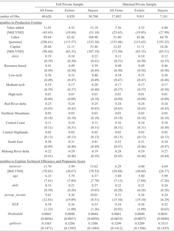
The left panel of Table 2 and Table 3 report the means of value added, labor, and capital for exiters, stayers, and all firms separately for private and state firms. Table 2 shows for private firms that the means of L, K, and Y for exiters are 42, 11, and 4, whereas those of stayers are 105, 23, and 13, where unit of capital and value added is million VND. Therefore, exiters use 40% and 48% of labor and capital to produce 31% of output compared with stayers. Table3 shows for state firms that means of L, K, and Y for exiters are 363, 114, 50, whereas those for stayers are 596, 217, 133. Therefore, exiters use 61% and 53% of labor and capital to produce 38% of output compared with stayers. These simple comparisons suggest that exiters are substantially smaller in production scale and seem to have lower productivity than stayers.
Next, we introduce variables which explain exit probability. They include five firm-specific variables (turnover, age, debt, wage income, capital labor ratio), two industry-specific variables (competition or concentration level, the presence of foreign firms within the industry), and four types of dummy variables (ownership, industries, regions, and years). Turnover in logarithm is used to represent firm size2 and it is expected
to reduce exit probability. Variable age is defined as the difference between the current and registration years3 and
it can also reduce exit probability. Consequently, large and old firms are less likely to exit due to the advantage of scale economies and their accumulated experiences (Jovanovic, 1982). Variable debt is defined as the ratio of total liabilities to total assets. While higher debt is likely to raise exit probability due to higher interest payments and likely bankruptcy (Tsionas and Papadogonas, 2006; Paul, Johnston, and Frengley, 2000), it might lower exit probability if debt is regarded as proxy for easier access to formal financial system (Hansen, Rand, and Tarp, 2009). Variable percap_income is defined as total labor compensation divided by labor input, and it is used in logarithm in the exit probability function. This variable might raise exit probability due to burdensome wage payments, while it might lower exit probability due to higher effort of employees, as discussed in Yang and Chen (2009). Capital labor ratio, KLR, can have a negative effect on exit probability because firms with more capital often have higher profitability, while it can have a negative effect as a result of factor intensity in the standard trade model (Frazer, 2005).
Industrial concentration (or competition) is proxied by the index Herfindahlj=ΣiSji2, where Sji denotes the
market share of firm i in the industry j in terms of turnover. Herfindahl is expected to reduce exit probability because its higher value means weaker market competition. Finally, spilloverj is defined as the sum of the turnover
of foreign firms in industry j divided by the sum of the turnover of all firms in the same industry. It may raise exit probability if domestic firms lose their market shares to competing foreign firms due to the “market stealing” effect (Aitken and Harrison, 1999). On the contrary, it may lower exit probability if domestic firms can imitate the better products of foreign firms and they devote more efforts to prevent falling behind these foreign firms (Caves, 1974; Javorcik, 2004).
The left panel of Table 2 and Table 3 also report the means of variables explaining exit probability for exiters, stayers, and all firms separately for private and state firms. In Table 2 (private firms), comparison of the two types of firms using the full sample shows that exiters have much smaller turnover, are younger, incur fewer liabilities, and pay lower wages, although they have similar characteristics for the other three variables (KLR, Herfindahl,
spillover). However, if we use the matched sample, these differences almost disappear. We can find a similar result
Table 2. Means of Variables over Full and Matched Samples: Private Firms
Full Private Sample Matched Private Sample
All Firms Exiters Stayers All Firms Exiters Stayers
Number of Obs. 40,620 9,920 30,700 17,092 9,911 7,181
Variables in Production Frontier
Value added 11.01 4.32 13.18 5.36 4.32 6.80 [Mill.VND] (45.65) (19.84) (51.10) (23.65) (19.85) (27.99) Labor 89.64 42.42 104.90 51.80 42.46 64.70 [persons] (296.61) (115.57) (333.38) (153.48) (115.62) (193.22) Capital 20.44 11.11 23.46 12.43 11.11 14.26 [Mill.VND] (98.44) (63.32) (107.19) (73.50) (63.35) (85.51) dsize 0.19 0.10 0.22 0.11 0.10 0.12 (0.39) (0.30) (0.41) (0.31) (0.30) (0.33) Resource-based 0.41 0.49 0.39 0.48 0.49 0.46 (0.49) (0.50) (0.49) (0.50) (0.50) (0.50) Low-tech 0.38 0.33 0.40 0.34 0.33 0.36 (0.49) (0.47) (0.49) (0.47) (0.47) (0.48) Medium-tech 0.19 0.17 0.20 0.17 0.17 0.17 (0.39) (0.37) (0.40) (0.37) (0.37) (0.38) High-tech 0.01 0.01 0.01 0.01 0.01 0.01 (0.09) (0.09) (0.10) (0.09) (0.09) (0.09)
Red River delta 0.25 0.24 0.25 0.24 0.24 0.24
(0.43) (0.43) (0.43) (0.43) (0.43) (0.43) Northern Mountains 0.03 0.03 0.03 0.03 0.03 0.03 (0.18) (0.18) (0.18) (0.18) (0.18) (0.18) Central Coast 0.11 0.10 0.11 0.10 0.10 0.10 (0.31) (0.31) (0.31) (0.31) (0.31) (0.30) Central Highlands 0.02 0.02 0.02 0.02 0.02 0.02 (0.13) (0.13) (0.13) (0.13) (0.13) (0.13) South East 0.38 0.31 0.41 0.32 0.31 0.34 (0.49) (0.46) (0.49) (0.47) (0.46) (0.47)
Mekong River delta 0.22 0.29 0.19 0.28 0.29 0.27
(0.41) (0.46) (0.39) (0.45) (0.46) (0.44)
Variables to Explain Technical Efficiency and Propensity Score
turnover 11.76 5.99 13.62 6.29 6.00 6.69 [Bill.VND] (70.85) (30.67) (79.53) (28.88) (30.69) (26.17) age 6.23 5.79 6.37 5.88 5.80 5.99 (7.61) (7.04) (7.78) (7.13) (7.04) (7.26) debt 0.33 0.21 0.37 0.22 0.21 0.24 (8.39) (0.28) (9.65) (0.28) (0.28) (0.28) percap_income 9.61 8.36 10.01 8.31 8.36 8.24 (12.01) (19.09) (8.51) (15.10) (19.10) (6.29) KLR 0.34 0.36 0.33 0.34 0.36 0.32 (1.22) (1.09) (1.26) (0.92) (1.09) (0.63) Herfindahl 0.0043 0.0040 0.0044 0.0041 0.0040 0.0041 (0.0056) (0.0057) (0.0056) (0.0053) (0.0057) (0.0048) spillover 0.3363 0.3288 0.3388 0.3299 0.3289 0.3313 (0.1471) (0.1395) (0.1494) (0.1412) (0.1396) (0.1435) Note: Standard deviations are shown in parentheses and units are shown in brackets.
Table 3. Means of Variables over Full and Matched Samples: State Firms
Full State Sample Matched State Sample
All Firms Exiters Stayers All Firms Exiters Stayers
Number of Obs. 5,712 1,044 4,668 1,874 1,044 830
Variables in Production Frontier
Value added 117.71 50.09 132.85 54.73 50.14 60.50 [Mill.VND] (374.44) (116.91) (409.00) (123.70) (116.96) (131.54) Labor 553.35 363.32 595.88 385.31 363.64 412.57 [persons] (887.60) (543.74) (942.44) (564.88) (543.90) (589.41) Capital 197.68 113.52 216.52 116.23 113.63 119.50 [Mill.VND] (620.52) (230.94) (676.30) (236.77) (231.02) (243.90) dsize 0.69 0.54 0.72 0.56 0.54 0.58 (0.46) (0.50) (0.45) (0.50) (0.50) (0.49) Resource-based 0.25 0.31 0.23 0.30 0.31 0.30 (0.43) (0.46) (0.42) (0.46) (0.46) (0.46) Low-tech 0.49 0.44 0.50 0.44 0.44 0.45 (0.50) (0.50) (0.50) (0.50) (0.50) (0.50) Medium-tech 0.25 0.24 0.25 0.24 0.24 0.24 (0.43) (0.42) (0.44) (0.42) (0.42) (0.43) High-tech 0.02 0.02 0.02 0.02 0.02 0.01 (0.13) (0.13) (0.13) (0.12) (0.13) (0.11)
Red River delta 0.37 0.40 0.37 0.39 0.40 0.38
(0.48) (0.49) (0.48) (0.49) (0.49) (0.48) Northern Mountains 0.10 0.11 0.10 0.11 0.11 0.12 (0.30) (0.32) (0.30) (0.32) (0.32) (0.32) Central Coast 0.17 0.18 0.17 0.18 0.18 0.18 (0.37) (0.38) (0.37) (0.38) (0.38) (0.39) Central Highlands 0.03 0.04 0.03 0.04 0.04 0.04 (0.17) (0.20) (0.16) (0.20) (0.20) (0.21) South East 0.24 0.18 0.25 0.18 0.18 0.19 (0.42) (0.38) (0.43) (0.38) (0.38) (0.39)
Mekong River delta 0.09 0.10 0.09 0.09 0.10 0.09
(0.28) (0.29) (0.28) (0.29) (0.29) (0.29)
Variables to Explain Technical Efficiency and Propensity Score
turnover 101.04 53.83 111.60 50.39 53.89 46.00 [Bill.VND] (282.72) (160.03) (302.47) (137.13) (160.10) (101.00) age 21.62 19.21 22.16 19.65 19.21 20.19 (13.19) (13.06) (13.16) (13.13) (13.07) (13.20) debt 0.65 0.67 0.64 0.67 0.67 0.67 (0.37) (0.46) (0.35) (0.46) (0.46) (0.46) percap_income 15.16 11.68 15.94 11.76 11.69 11.84 (19.41) (8.22) (21.04) (8.04) (8.21) (7.83) KLR 0.41 0.40 0.41 0.40 0.40 0.39 (0.71) (0.66) (0.72) (0.69) (0.66) (0.72) Herfindahl 0.0060 0.0056 0.0061 0.0056 0.0056 0.0057 (0.0050) (0.0047) (0.0051) (0.0047) (0.0047) (0.0047) spillover 0.3283 0.3397 0.3257 0.3400 0.3398 0.3402 (0.1983) (0.1853) (0.2010) (0.1921) (0.1854) (0.2002) Note: Standard deviations are shown in parentheses and units are shown in brackets.
3. Empirical Analysis
3.1. MethodsAssuming private and state firms possess different production technology, we specify and estimate two Cobb-Douglas SPFs separately for these firms. Specifically, the SPF has two inputs (labor Lit and capital Kit) and one
output (value added Yit) for firm i ( = 1, …, n) and year t ( = 2000, …, 2004):
lnYit = β0 + β1lnLit + β2lnKit + αexitit + β3dsizeit + ΣgEG βgndindustryig
+ ΣrER βrdregionir + Σs βsdyears + vit - uit , (1)
where dsize denotes firm size dummy taking the value 1 if the firm is classified as large scale, dyears denotes time
dummy variables for year s = 2001, ... , 2005, with 2000 chosen as the base year; dregionir denotes regional
dummy variables for firm i in region r with R denoting a regional set which includes five out of the six regions mentioned above (Red River delta is chosen as the base group); dindustryig denotes industrial dummy variables for
firm i in industrial group g with G denoting an industrial set which includes three out of four industrial groups as introduced in the subsection 2.2 (medium-tech is chosen as the base group). Note that subscript j for industries is omitted from variables (except for dindustryig) to simplify notations, which means that their coefficients are
common to all industries. In equation (1), production technology between exiting and staying firms differs only in the intercept, as the dummy variable exitit shows. A negative coefficient α of exitit means that exiting firms have a
lower production frontier than staying firms do, with other things being equal. We assume that vit is a normal
random variable with mean zero and constant variance σv2 and that non-negative technical inefficiency uit follows a
half normal distribution with variance σu2.
Caudill, Ford, and Gropper (1995) emphasize that the heteroskedasticity of inefficiency u can substantially affect the estimated TE index. Then, we assume that inefficiency u has the following heteroskedastic function4:
lnσu2 = δ0 + Σs δsdyears + δ1dsizeit + δ2ageit + δ3debtit
+ δ4dpercap_incomeit + δ5Herfindahljt + δ6spilloverjt. (2)
To obtain a matched stayer for each exiter, we specify the following probit model: exitit =
{
1 for exiting firms if Iit*> 0
0 for continuing firms if I*it<_ 0
Iit* = γ0 + γ1ln (turnover)it + γ2ageit + γ3debtit + γ4ln (percap_incomeit )
+ γ5ln (KLR)it + γ6Herfindahlit + γ7spilloverit
+ ΣgEG γgdindustryig + ΣrER γr dregionir + Σs γs dyears + eit , (3)
where eit is a standard normal variable. Matched sample is constructed by propensity score matching (PSM)
method of Mayen, Balagtas and Alexander (2010). First, we estimate the probit model (3) using data for all firms and predict probability Pr (exit = 1) to exit for each firm. Next, we apply single-nearest-neighbor matching with pre-defined caliper and with replacement5 to reduce the bias. After this procedure, each exiter is matched with a
stayer with similar (i.e., closest) propensity score. Other unmatched stayers are dropped for the sample (Dehejia and Wahba, 2002).
For private and state firms separately, we jointly estimate the SPF (1) and the variance function (2) using the maximum likelihood method in two ways. First, we estimate them using data on all exiters and stayers by ignoring endogeneity of exitit. Second, we estimate them using data on all exiters and their matched stayers to allow for the
endogeneity of exitit. After estimating the SPF and variance function, we follow Battese and Coelli (1988) to
TE = E [exp (-u) |Y] = {Φ [(u*/σ
*) - σ*]/Φ (u*/σ*)} exp [(σ*2 /2) - u*], (4)
where u*=- (ν-u) σ
u2/σ2, σ*2 = σu2σν2/σ2, and σ2= σu2 + σν2. Φ denotes the cumulative distribution function of
the standard normal variable.
3.2. Estimated Parameters of Exit Probability and Characteristics of Matched Samples
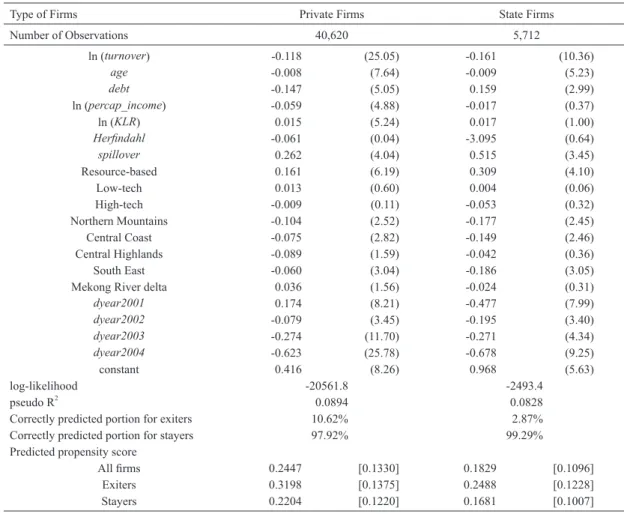
Estimation results of the probit model (3) for private and state firms are presented in Table 4. For private firms, the probit model has pseudo R2 at 0.089 and correctly predicts exit decision for 98% of stayers and for 11% of exiters.
Similarly, for state firms, the probit model has pseudo R2 of 0.083 and correctly predicts exit decision for 99% of
stayers and 3% for exiters. Most coefficients are estimated significantly at the 5% level.
Private firms tend to exit the market if they have higher values of capital intensity (KLR), they face more presence of foreign firms (spillover), or they have the resource-based industry membership (resource-based dummy). Conversely, they tend to stay in the market if they have larger production scale (turnover), they are older (age), they have more liabilities (debt), or they pay higher wage (percap_income). Furthermore, private firms in the Northern Mountains, Central Coast, and South East regions are less likely to exit, and exit probability of
Table 4. Estimated Coefficients of Probit Model of Firm Exit
Type of Firms Private Firms State Firms
Number of Observations 40,620 5,712 ln (turnover) -0.118 (25.05) -0.161 (10.36) age -0.008 (7.64) -0.009 (5.23) debt -0.147 (5.05) 0.159 (2.99) ln (percap_income) -0.059 (4.88) -0.017 (0.37) ln (KLR) 0.015 (5.24) 0.017 (1.00) Herfindahl -0.061 (0.04) -3.095 (0.64) spillover 0.262 (4.04) 0.515 (3.45) Resource-based 0.161 (6.19) 0.309 (4.10) Low-tech 0.013 (0.60) 0.004 (0.06) High-tech -0.009 (0.11) -0.053 (0.32) Northern Mountains -0.104 (2.52) -0.177 (2.45) Central Coast -0.075 (2.82) -0.149 (2.46) Central Highlands -0.089 (1.59) -0.042 (0.36) South East -0.060 (3.04) -0.186 (3.05)
Mekong River delta 0.036 (1.56) -0.024 (0.31)
dyear2001 0.174 (8.21) -0.477 (7.99) dyear2002 -0.079 (3.45) -0.195 (3.40) dyear2003 -0.274 (11.70) -0.271 (4.34) dyear2004 -0.623 (25.78) -0.678 (9.25) constant 0.416 (8.26) 0.968 (5.63) log-likelihood -20561.8 -2493.4 pseudo R2 0.0894 0.0828
Correctly predicted portion for exiters 10.62% 2.87%
Correctly predicted portion for stayers 97.92% 99.29%
Predicted propensity score
All firms 0.2447 [0.1330] 0.1829 [0.1096]
Exiters 0.3198 [0.1375] 0.2488 [0.1228]
経済経営論集 第 24 巻第 2 号
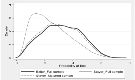
private firms started decreasing since 2002. Results for state firms are very similar to those for private firms. We use these parameter estimates to compute the propensity score or the predicted probability of being an exiter for each firm. We then select for each exiter a stayer which has the propensity score closest to that of the exiter. Figure 1 shows the kernel densities of propensity scores for exiters, stayers, and matched stayers. As expected, for both private and state firms, the distribution of stayers is skewed towards zero, while that of matched stayers gets very close to the distribution of exiters.
Before estimating the SPF and variance function using matched sample, we briefly examine characteristics of this sample, which are shown in the right panel of Table 2 and Table 3. The resulting matched sample, which is composed of exiters and matched stayers, includes 17,092 (1,874) firms for private (state) firms. The matched stayers have similar characteristics to exiters for all variables in Tables 2 and 3. In Table 2, for example, the means
Figure 1. Kernel Densities of Exit Probability for Exiters and Stayers
probability of being an exiter for each firm. We then select for each exiter a stayer which has the
propensity score closest to that of the exiter. Figure 1 shows the kernel densities of propensity
scores for exiters, stayers, and matched stayers. As expected, for both private and state firms,
the distribution of stayers is skewed towards zero, while that of matched stayers gets very close
to the distribution of exiters.
Figure 1. Kernel Densities of Exit Probability for Exiters and Stayers
Private Firms
State Firms
Source: The author’s calculation based on the microdata of the GSO for 2000-2004
0 1 2 3 4 De n s it y 0 .2 .4 .6 .8 Probability of Exit
Exiter_Full sample Stayer_Full sample Stayer_Matched sample 0 1 2 3 4 5 D e nsi t y 0 .2 .4 .6 .8 Probability of Exit
Exiter_Full sample Stayer_Full sample Stayer_Matched sample
Private Firms
State Firms
probability of being an exiter for each firm. We then select for each exiter a stayer which has the
propensity score closest to that of the exiter. Figure 1 shows the kernel densities of propensity
scores for exiters, stayers, and matched stayers. As expected, for both private and state firms,
the distribution of stayers is skewed towards zero, while that of matched stayers gets very close
to the distribution of exiters.
Figure 1. Kernel Densities of Exit Probability for Exiters and Stayers
Private Firms
State Firms
Source: The author’s calculation based on the microdata of the GSO for 2000-2004
0 1 2 3 4 De n s it y 0 .2 .4 .6 .8 Probability of Exit
Exiter_Full sample Stayer_Full sample Stayer_Matched sample 0 1 2 3 4 5 D e nsi t y 0 .2 .4 .6 .8 Probability of Exit
Exiter_Full sample Stayer_Full sample Stayer_Matched sample
of L, K, and Y are 65, 14, and 7 for matched stayers, which are much closer to those for exiters (42, 11, and 4) than those for stayers (105, 23, 13). Similar results are shown in Table 3. Other variables, age, debt, and percap_income for matched stayers are also closer to those of exiters, as shown in the two tables.
3.3. Estimated Parameters of the SPF and the Variance Function
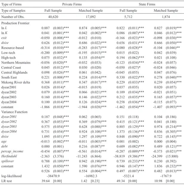
Table 5 presents estimated parameters of the SPF (1) and the variance function (2) over full sample of and matched sample separately for private and state firms. For private firms, the coefficient of exitit, which represents
technology difference between exiters and stayers, is negative for both full and matched samples. However, this difference is found to be statistically insignificant once we control for endogeneity of exit decision, which suggests
Table 5. Estimated Parameters of Stochastic Production Frontiers over Full and Matched Samples
Type of Firms Private Firms State Firms
Type of Samples Full Sample Matched Sample Full Sample Matched Sample
Number of Obs. 40,620 17,092 5,712 1,874 Production Frontier ln L 0.887 (0.003)*** 0.874 (0.005)*** 0.822 (0.011)*** 0.827 (0.019)*** ln K 0.041 (0.001)*** 0.042 (0.002)*** 0.086 (0.007)*** 0.046 (0.012)*** exit -0.050 (0.008)*** -0.012 (0.010) -0.166 (0.023)*** -0.098 (0.030)*** dsize 0.626 (0.012)*** 0.686 (0.022)*** 0.656 (0.031)*** 0.666 (0.050)*** Resource-based -0.314 (0.010)*** -0.283 (0.017)*** -0.080 (0.028)** -0.104 (0.046)** Low-tech -0.200 (0.009)*** -0.195 (0.015)*** 0.015 (0.022) 0.042 (0.039) High-tech 0.075 (0.032)** 0.135 (0.054)** 0.194 (0.062)*** 0.021 (0.108) Northern Mountains -0.056 (0.020)** -0.032 (0.033) -0.123 (0.034)*** -0.024 (0.057) Central Coast 0.045 (0.012)*** 0.030 (0.020) -0.050 (0.027)* -0.024 (0.046) Central Highlands 0.098 (0.026)*** 0.061 (0.042) -0.045 (0.055) 0.047 (0.076) South East 0.221 (0.008)*** 0.224 (0.014)*** 0.330 (0.022)*** 0.278 (0.040)*** Mekong River delta 0.368 (0.011)*** 0.347 (0.017)*** 0.229 (0.033)*** 0.239 (0.054)***
dyear2001 0.026 (0.014)* -0.015 (0.019) 0.037 (0.035) 0.020 (0.057) dyear2002 0.079 (0.014)*** 0.066 (0.021)*** 0.109 (0.034)*** -0.021 (0.051) dyear2003 0.160 (0.014)*** 0.146 (0.022)*** 0.212 (0.035)*** 0.165 (0.057)*** dyear2004 0.100 (0.014)*** 0.126 (0.024)*** 0.258 (0.036)*** -0.115 (0.077) constant -1.866 (0.018)*** -1.944 (0.028)*** -1.462 (0.054)*** -1.407 (0.093)*** Variance Function dyear2001 0.187 (0.048)*** 0.062 (0.065) 0.151 (0.118) 0.104 (0.186) dyear2002 0.367 (0.053)*** 0.369 (0.079)*** 0.415 (0.121)*** 0.041 (0.180) dyear2003 0.575 (0.054)*** 0.628 (0.088)*** 0.885 (0.129)*** 0.974 (0.214)*** dyear2004 0.731 (0.054)*** 0.924 (0.108)*** 1.373 (0.136)*** 0.836 (0.305)*** dsize 1.095 (0.051)*** 1.297 (0.109)*** 0.848 (0.090)*** 0.722 (0.145)*** age -0.013 (0.002)*** -0.011 (0.003)*** 0.001 (0.002) 0.000 (0.004) debt 0.000 (0.001) 0.216 (0.087)** 0.609 (0.082)*** 0.489 (0.121)*** percap_income -0.454 (0.007)*** -0.561 (0.014)*** -0.287 (0.009)*** -0.373 (0.021)*** Herfindahl -2.363 (3.376) -11.243 (6.864) -38.819 (9.386)*** -24.399 (15.880) spillover 0.788 (0.109)*** 0.942 (0.190)*** 0.739 (0.233)*** 0.230 (0.392) constant 1.432 (0.050)*** 1.590 (0.076)*** 0.946 (0.147)*** 1.836 (0.232)*** 0.526 (0.003)*** 0.554 (0.004)*** 0.497 (0.007)*** 0.482 (0.013)*** log-likelihood -38470.9 -16982.3 -5321.4 -1767.9 LR test 39.64 [0.00] 1.42 [0.23] 49.34 [0.00] 10.98 [0.00]
the importance of the use of PSM method. On the other hand, for state firms, the coefficient of exitit is statistically
negative for both full and matched samples and the difference is statistically significant even after controlling for the endogeneity.
For private firms, estimated production elasticities of labor and capital are similar between the full and matched samples. For state firms, estimated production elasticity of labor is similar between these samples, while that of capital is different (0.09 and 0.05). For other coefficients, most of them are similar between the full and matched samples both for private and state firms if we focus on statistically significant coefficients. The only difference can be found for the coefficient of high-tech industry dummy for private firms and 2003 and 2004 year dummies for state firms.
3.4. Comparison of Production Frontiers and Technical Efficiency
The upper panel of Table 6 presents predicted outputs (i.e., deterministic production frontiers) for exiters and stayers over the full and matched samples, where unit is million VND. The average production frontiers of exiters and stayers over the full sample are higher than those over the matched sample for both private and state firms. The difference is 100% for private exiters, 110% for private stayers, 72% for state exiters, and 84% for state stayers. The difference between the two types of samples is the highest in 2002 for private exiters and stayers (100% and 107%), in 2004 for state exiters and stayers (144% and 161%). These higher predicted outputs over the full sample come from overestimation by ignoring endogenous firm exit in the estimation of the SPFs.
Focusing on the result over the matched sample, the predicted output shows the same production frontiers between private exiters and stayers and slightly different production frontiers between state exiters and stayers, reflecting the estimated coefficients of the dummy variable, exitit, for private and state firms. Furthermore, private
exiters and stayers are found to upgrade their production technology annually, e.g., 100% (from 4.6 to 9.2) for exiters and 102% (from 4.6 to 9.3) for stayers from 2000 to 2004. On the other hand, state exiters and stayers reached their peak in 2003 (from 65.5 in 2000 to 90.4 in 2003, and 72.2 to 99.8 for the same years) and turned back to the level in 2000 (65.5 and 72.3) after a slight decrease in 2001-2002.
Table 6. Predicted Outputs and Technical Efficiency over Full and Matched Samples
Type of Samples Full Sample Matched Sample
2000 2001 2002 2003 2004 Total 2000 2001 2002 2003 2004 Total Predicted Outputs Private-Firm Sample Exiters 8.4 9.8 13.6 16.1 14.5 12.6 4.6 4.9 6.8 8.5 9.2 6.3 Stayers 8.8 10.3 14.3 16.9 15.3 13.2 4.6 5.0 6.9 8.6 9.3 6.3 State-Firm Sample Exiters 85.9 95.0 113.3 145.6 159.8 117.1 65.5 64.1 60.9 90.4 65.5 68.2 Stayers 101.5 112.2 133.8 172.0 188.6 138.3 72.2 70.7 67.2 99.8 72.3 75.3 Predicted Technical Efficiency
Private-Firm Sample Exiters 0.59 0.58 0.65 0.67 0.69 0.62 0.63 0.64 0.69 0.72 0.73 0.67 Stayers 0.64 0.67 0.70 0.72 0.73 0.70 0.62 0.68 0.71 0.72 0.74 0.69 State-Firm Sample Exiters 0.58 0.57 0.56 0.58 0.52 0.57 0.60 0.59 0.63 0.63 0.65 0.61 Stayers 0.64 0.65 0.66 0.66 0.66 0.65 0.60 0.62 0.67 0.67 0.65 0.64 Note: Full sample is the original sample for all firms. Matched sample is that with Stayers repeatedly used in matching.
Caliper width is defined as one-quarter of the standard deviation of the predicted propensity score (exit probability) for all firms in each of the corresponding full samples. Unit of predicted output is million VND.
The lower panel of Table 6 presents predicted TEs for exiters and stayers over the full and matched samples. Average TE of exiters is lower than that of stayers for both these samples and the difference is larger over the full sample. For example, the difference for private firms is 0.08 and 0.02 over the full and matched samples, and that for state firms is 0.08 and 0.03 over these samples. TEs for private and state exiters over the full samples are smaller than those over the matched sample, whereas there is almost no TE difference for private and state stayers over the two samples. Focusing on the matched sample, the estimated TEs show an increasing trend for all types of firms by ownership (private or state) and by exit status (exiters or stayers). Private exiters and stayers respectively gained 10% and 12% of their TE between 2000 and 2004, whereas both state exiters and stayers gained 5% of their TE for the same period.
4. Summary and Conclusions
This analysis uses data on individual manufacturing firms for 2000–2004 to examine the effect of endogeneity of firmsʼ exit decision on their production frontiers. For this purpose, it estimates Cobb-Douglas production frontiers with different intercepts for exiting and staying firms separately for private and state firms.
The empirical results indicate some estimation bias from endogenous exit decision of firms. When we use data on all private firms to estimate the SPF, exiting firms have a 5% lower production frontier and exiting state firms have a 15% lower production frontier. On the other hand, when we use data on exiting and matched staying private firms, only exiting state firms show a significantly lower frontier (9%). Furthermore, estimation with the full sample overestimates some parameters of the SPF than that with the matched sample, especially for state firms. In terms of TE, the difference is larger for the full sample than for the matched sample: Exiting private firms are less technically efficient by 0.08 (0.02), and exiting state firms are less technically efficient by 0.08 (0.03) over the full (matched) sample.
Comparison of the results over the full and matched samples in terms of the SPF parameters, predicted outputs, and TEs shows that the PSM method can correct the bias from endogenous firm exit more effectively for private firms than for state firms. Such different results between the two types of samples imply the importance to consider the firm exit endogeneity in estimating the SPF, although the PSM method seems to correct this endogeneity only partially.
Our model does not capture the effect of the unobservable productivity on the exit decision and their interactions in the SPF specification. In the future study, we should reconsider this effect by employing different methods, which include a simultaneous estimation of the SPF and firm exit probit model.
Note
1 Many private firms do not report fringe benefits that are included in total labor compensation defined in this study. We replace missing values of fringe benefits with zero for private firms because most of them are unlikely to pay fringe benefits. Furthermore, some private firms report fixed assets to be zero. For these firms, fixed assets are replaced with one tenth of the smallest positive value of fixed assets to estimate a Cobb-Douglas production frontier.
2 This measurement in terms of turnover is used only in the probit model for firm exit probability. In the SPF and the variance function of technical inefficiency, we use the dummy variable dsize for firm size to categorize “large scale” and “small scale” firms.
3 We dropped from our sample firms which report the registration year to be zero, smaller than 1945, or larger than the current year.
Rubin (1985) for how to define the caliper width. We, in the preliminary analysis, construct the matched sample in two ways with and without pre-defined caliper and the two give the same estimation results. Therefore, we decide to report the results of the matched sample with pre-defined caliper in the body of the paper.
References
Ahuja, G. and S.K. Majumdar (1998), “An assessment of the performance of Indian state-owned enterprises,”
Journal of Productivity Analysis, Vol.9, No.2, pp.113-132.
Aitken, B.J. and A.E. Harrison (1999), “Do domestic firms benefit from direct foreign investment? Evidence from Venezuela,” American Economic Review, Vol.89, No.3, pp. 605-618.
Battese, G.E. and T.J. Coelli (1988), “Prediction of firm-level technical efficiencies with a generalized frontier production function and panel data,” Journal of Econometrics, Vol.38, No.3, p.387-399.
Caudill, S.B., J.M. Ford, and D.M. Gropper (1995), “Frontier estimation and firm-specific inefficiency measures in the presence of heteroskedasticity,” Journal of Business and Economic Statistics, Vol.13, No.1, pp.105-111. Caves, R.E. (1974), “Multinational firms, competition and productivity in host-country markets. Economica,
Vol.41, pp.176-193.
Coelli, T.J., D.S.P. Rao, C.J. OʼDonnell, and G.E. Battese (2005), An Introduction to Efficiency and Productivity
Analysis, 2nd edition, Springer.
Dehejia, R.H. and S, Wahba (2002), “Propensity score-matching methods for nonexperimental causal studies,”
Review of Economic and Statistics, Vol.84, No.1, pp.151-161.
Frazer, G. (2005), “Which firms die? A look at manufacturing firm exit in Ghana,” Economic Development and
Cultural Change, Vol.53, No.3, pp.585-617.
Friedman, J. (2004), “Firm ownership and internal practices in a transition economy,” Economics of Transition, Vol.12, No.2, pp.333-366.
General Statistics Office (GSO) of Vietnam (2006), Vietnamese Industry in 20 Years of Renovation and
Development, Statistical Publishing House.
General Statistics Office (GSO) of Vietnam (2010), Enterprises in Vietnam during the First Nine Years of 21st
Century, Statistical Publishing House.
Ghosh, M. and J. Whalley (2008), “State owned enterprises, shirking and trade liberalization,” Economic
Modelling, Vol.25, No.6, pp.1206-1215.
Hansen, H., J. Rand, and F. Tarp (2009), “Enterprise growth and survival in Vietnam: Does government support matter?,” Journal of Development Studies, Vol.45, No.7, pp.1048-1069.
Javorcik, B.S. (2004), “Does foreign direct investment increase the productivity of domestic firm? In search of spillovers through backward linkages,” American Economic Review, Vol.94, No.3, pp.605-627.
Jovanovic, B. (1982), “Selection and the evolution of industries,” Econometrica, Vol.50, No.3, pp.649-670. Kumbhakar, S.C., E.G. Tsionas, and T. Sipiläinen (2009), “Joint estimation of technology choice and technical
efficiency: An application to organic and conventional dairy farming,” Journal of Productivity Analysis, Vol.31, No.3, pp.151-161.
Leung, S.E. (2010), “Vietnam: an economic survey,” Asian-Pacific Economic Literature, Vol. 24, No.2, pp.83-103. Mayen, C.D., J.V. Balagtas, and C.E. Alexander (2010), “Technology adoption and technical efficiency: Organic
and conventional dairy farms in the United States,” American Journal of Agricultural Economics, Vol.92, No.1, pp.181-195.
MoIT (Ministry of Industry and Trade of Vietnam) and UNIDO (United Nations Industrial Development Organization) (2011). Vietnam Industrial Competitiveness Report 2011.
Nguyen, T.T. and M.A. van Dijk (2012), “Corruption, growth, and governance: Private vs. state-owned firms in Vietnam,” Journal of Banking and Finance, Vol.36, No.12, pp.2935-2948.
Nguyen, T.V., N.T.B. Le, and S.E. Bryant (2013), “Sub-national institutions, firm strategies, and firm performance: A multilevel study of private manufacturing firms in Vietnam,” Journal of World Business, Vol.48, No.1, pp.68-76.
Olley, G.S. and A. Pakes (1996), “The dynamics of productivity in the telecommunications equipment industry,”
Econometrica, Vol.64, No.6, pp.1263-1297.
Paul, C.J.M, W.E. Johnston, and G.A.G. Frengley (2000), “Efficiency in New Zealand sheep and beef farming: The impacts of regulatory reform,” Review of Economics and Statistics, Vol.82, No.4, pp.325-337.
Pham, H.T., T.L. Dao, and B. Reilly (2010), “Technical efficiency in the Vietnamese manufacturing sector,”
Journal of International Development, Vol.22, No.4, pp.503-520.
Rand, J. and N. Torm (2012), “The benefits of formalization: Evidence from Vietnamese manufacturing SMEs,”
World Development, Vol.40, No.5, pp.983-998.
Sari, N. (2003), “Efficiency outcomes of market concentration and managed care,” International Journal of
Industrial Organization, Vol.21, No.10, pp.1571-1589.
Shiferaw, A. (2009), “Survival of private sector manufacturing establishments in Africa: The role of productivity and ownership,” World Development, Vo.37, No.3, pp.572-584.
Söderbom, M. and F. Teal (2004), “Size and efficiency in African manufacturing firms: Evidence from firm-level panel data,” Journal of Development Economics, Vol.73, No.1, pp.369-394.
Söderbom, M., F. Teal, and A. Harding (2006), “The determinants of survival among African manufacturing firms,”
Economic Development and Cultural Change, Vol.54, No.3, pp.533-555.
Steer, L. and K. Sen (2010), “Formal and informal institutions in a transition economy: The case of Vietnam,”
World Development, Vol.38, No.1, pp.1603-1615.
Suyanto, S., R.A. Salim, and H. Bloch (2009), “Does foreign direct investment lead to productivity spillover? Firm level evidence from Indonesia," World Development, Vol.37, No.12, pp.1861-1876.
Tsionas, E.G. and T.A. Papadogonas (2006), “Firm exit and technical inefficiency,” Empirical Economics, Vol.31, No.2, pp.535-548.
Vu, Q.N. (2003), “Technical efficiency of industrial state-owned enterprises in Vietnam,” Asian Economic Journal, Vol.17, No.1, pp.87-101.
Vu, T.B.L. (2014), “Small Privately-Owned and Large State-Owned Manufacturing Firms in Vietnam: A Productivity Comparison for 2000-2005,” Economic Science 62, pp.45-67.
Vu, T.B.L. and T. Sonoda (2015), “Does Firm Size Matter for the Effect of Productivity on Firmsʼ Market Exit? Evidence from Vietnamese Manufacturing Firms,” Empirical Economics Letters 14 (3).
Yang, C.H. and K.H. Chen (2009), “Are small firms less efficient?,” Small Business Economics, Vol.32, No.4, pp.375-395.