Direct Boundary Element Method for Calculation of Oseen Flow Past a Circular Cylinder in Case of Linear Variation
Ghulam Muhammad
1, Nawazish Ali Shah
2, and Muhammad Mushtaq
21
Department of Mathematics, GCS, Lahore, Pakistan
2
Department of Mathematics, University of Engineering & Technology, Lahore – 54890, Pakistan
* Corresponding Author: [email protected]
Abstract: In present paper, direct boundary element method (DBEM) has been applied to calculate Oseen flow past a circular cylinder in case of linear variation. The boundary of the circular cylinder is discretized into constant boundary elements over which the velocity distribution is calculated. The calculated results are also compared with exact results.
[Ghulam Muhammad, Nawazish Ali Shah, and Muhammad Mushtaq. Direct Boundary Element Method for Calculation of Oseen Flow Past a Circular Cylinder in Case of Linear Variation. Academ Arena 2017;9(2):74- 81]. ISSN 1553-992X (print); ISSN 2158-771X (online). http://www.sciencepub.net/academia. 7.
doi:10.7537/marsaaj090217.07.
Keywords: Direct boundary element method, Oseen flow, Circular cylinder, Linear variation.
Introduction
Boundary element method is a numerical technique used to solve the different types of problems today facing in science and technology. The well-known computational methods such as finite difference method (FDM) and finite element method (FEM) are very costly and time- consuming because in these methods the whole domain under study is discretised into a number of block-type elements, whereas in boundary element method the process of discretisation takes place on the surface of body.
Which considerably reduces the size of system of equations resulting the reduction in data and that is perquisite to run a computer program efficiently. In other words, boundary element methods are superior in several aspects to other computational methods because of their surface modeling approach. That is why, the complicated structures can be more easily modeled by these methods and are therefore preferred by engineers. The results of boundary element methods are more accurate and reliable than those of classical methods. which establishes the fact that these methods (BEMs) are time-saving, accurate, efficient and economical techniques as compared to other numerical techniques (Mushtaq, M; 2008, 2009, 2011). These salient features of BEMs make them popular in communities of engineering and science.
Such methods are essentially the methods for solving the partial differential equations arising in wide range of fields, e.g., fluid mechanics, solid and fracture mechanics, heat transfer and electromagnetic theory, potential theory, elasticity, elastostatics and elastodynamics, etc. as detailed in Brebbia and Walker, (1980). Furthermore, the area of their applications is increasing day to day. Boundary element methods have been classified into direct and
indirect methods. The direct method is in the form of a statement which gives the values of unknown variables at the field point under discussion in terms of a complete set of the entire boundary data. whereas the indirect method is based on the distribution of sources or doublets over the boundary of the body and calculates such distribution in terms of the solution of an integral equation. The first work on flow field calculations around three-dimensional bodies was probably done by Hess and Smith, (1962 & 1967).
The direct boundary element method (DBEM) for potential flow calculations around objects was first applied in past by Morino et al (1975). In recent past, the direct boundary element methods have been applied by the author himself for flow field calculations around two- and three-dimensional objects (Muhammad, G; 2008, 2010).
Calculation of Oseen Flow Past a Circular Cylinder
Figure 1
Boundary element methods are applied for both
problems of exterior and interior flows in two
dimensional space.. In this section, direct boundary
element method is used to calculate the Oseen’s flow
around a circular cylinder. A circular cylinder of radius ‘a’ is held fixed in a uniform stream of incompressible viscous fluid flowing steadily around it and let the centre of a cylinder be taken as origin and U
sbe the velocity of uniform stream in the positive.
x – direction as given in figure 1 (Shah, 2008).
The hydrodynamical equations are (Lamb, 1932).
U
s u
x = – 1
p
x + v
2u U
s v
x = – 1
p
y + v
2v
(1)
u
x + v
y = 0 (2)
Also
2p = 0 (3)
and p = U
s
x (4`)
The relations for the velocity components are (Milne Thomson, 1968) and (Lamb, 1932).
u =
x + 1 2k χ
x – χ v =
y + 1 2k χ
y
(5)
where k is an inertia coefficient.
Also, we know that
2 = 0 (6)
Now u
x =
2
x
2+ 1 2k
2χ
x
2– χ
x
u
y =
2
y
2+ 1 2k
2χ
y
2Using these relations in equation (2), we get
2
x
2+ 1 2k
2χ
x
2– χ
x –
2
y
2+ 1 2k
2χ
y
2= 0
2
x
2+
2
y
2+ 1 2k
2χ
x
2+
2χ
y
2– χ
x = 0
2 + 1 2k
2 –
x = 0 Since
2 = 0
1 2k
2 – 2k
x = 0 or
2 – 2k
x = 0
2– 2k
x = 0 (7)
Let the appropriate solution of equation (7) for small values of kr be
= − C (1 + k x)
+ ln 1 2 k r where γ is Euler constant.
Let us assume
= – U
sx + A
0ln r + A
1
x ln r + …….
so that the boundary conditions u = 0, v = 0 are satisfied on the boundary of a circular cylinder.
x = −C k
+ ln 1
2 k r − C ( 1 + k x )
x r
21
2 k
x
= − C 2 k
k
+ ln 1
2 k r + x r
2+ k x
2r
21
2 k
x – = − C
2 k
k
+ ln 1
2 k r + x r
2+ k x
2r
2– C (1 + k x )
+ ln 1 2 k r
(8) Also
x = – U
s+ A
0
x ( ln r ) + A
1
2 x
2(ln r) + ….
(9) Similarly,
y = −C ( 1 + k x )
y r
21
2 k
y = − C 2 k
y
r
2+ k x y r
2= − C 2 k
y (ln r) – 1
2 k r
2
2 x y (ln r) + ….
(10) and
y = A
0
y ( ln r ) + A
1
2 x y ( ln r ) + …….
(11) Using the equations (8), (9), (10) and (11) in equation (5), we have
u = – U
s− C
1
2 – – ln 1
2 k r +
A
0− C 2 k
x ( ln r ) +
A
1+ C
4 r
2
2 x
2( ln r ) + ……. (12) v = A
0
y ln r + A
1
2 x y ln r + …….
– C 2 k
y ln r + C 4 r
2
2 x y ln r + …….
or v =
A
0– C 2 k
y ln r +
A
1+ C
4 r
2
2 x y ln r
+……….. (13)
Boundary conditions are u = 0, v = 0, for r = a
Using the above boundary conditions in the equations
(12) and (13), we obtain
0 = – U
s− C
1
2 – – ln 1
2 k a +
A
0− C 2 k
x ( ln a ) +
A
1+ C
4 a
2
2 x
2( ln r ) + …….
and 0 =
which give on comparison – U
s− C
1
2 – – ln 1
2 k a = 0, A
0− C
2 k = 0 and A
1+ C
4 a
2= 0 or C = − 2 U
s1
2 – – ln 1 2 k a
A
0= C 2 k and A
1= − C
4 a
2Using these constants in equations (12) and (13), we obtain
u = – U
s− C
1
2 – – ln 1
2 k r +
– C 2 k + C
2 k
x ( ln r ) +
C 4 a
2– C
4 r
2
2 x
2( ln r )
= − U
s(14)
v = C
4 ( r
2– a
2)
2 x y ( ln r )
= U
s2( + ln 1 2 k a – 1
2 )
( r
2– a
2)
2 x y ( ln r ) (15) The magnitude of velocity is given by the relation
V = u
2+ v
2(16)
Now to approximate the surface of a circular cylinder, the coordinates of extreme points on the boundary elements are generated in a computer program as under.
The boundary of the cylinder can be divided into elements by the formula.
k= [ ( m + 2 ) – 2 k ]
m ,
k = 1, 2,……., m (17)
Then the coordinates of the extreme points of these m elements are calculated from
x
k= a cos
k
y
k= a sin
kk = 1, 2,……., m
(18) Take m = 8 and a = 1.
Linear Variation
Next the case is considered in which the boundary of the circular cylinder is divided into linear elements. In this case the nodes where the boundary conditions are specified are at the intersection of the elements (Muhammad, G 2008).
The figure 2 shows the discretization of the circular cylinder into 8 linear boundary elements.
Figure 2
The discretization of the surface of a circular cylinder is given in figure 2.
The mid-node coordinates over every element are defined by the formula.
x
m= x
k+ x
k + 1
2 y
m= y
k+ y
k + 12
k, m = 1, 2,…, 8
(19) The coordinates of the extreme points of the elements and the coordinates of the mid – point of each element where the velocity will be calculated can be found from the equations (18) and (19) respectively. The reason for distributing the elements in this way is such that the velocities are calculated at the same values of in both figure 2 so that computed results could be easily compared.
Equation for the direct boundary element method is given by
c
i
i=
– 1 2
ln
1 r
n d + 1 2
–i
n
ln 1 r d (20)
Which can be in the discretised form as – c
i
i+ m j = 1
j– i
n
1 2 ln 1
r d +
= m
j = 1
j
1 2 ln 1
r d (21)
Since and
n vary linearly over the element their values at any point on the element can be defined in terms of their nodal values and the interpolation functions N
1and N
2as
= [ N
1N
2]
1
2
n = [ N
1N
2]
1
n
2 n
(22)
The integrals along an element ‘j’ on the L.H.S.
of equation (21) can now written as
j – i
n
1 2 ln 1
r d =
j – i
[ N
1N
2]
n
1 2 ln 1
r d
1
2
= [ h 1 i j h 2
i j ]
1
2 Where
h k i j =
j – i N
k
n
1 2 ln 1
r d ,
k = 1, 2,………. (23)
The integrals on the R.H.S. of equation (21) can be written as
j
n
1 2 ln 1
r d
=
j[ N
1N
2]
1 2 ln 1
r d
1
n
2 n
= [ g 1 i j g 2
i j ]
1
n
2 n
where g k i j =
jN
k
1 2 ln 1
r d ,
k = 1, 2,……. (24)
Again, the integrals in equations (23) and (24) are evaluated numerically as before except for the element on which the fixed point ‘i’ is lying. For this element, the integrals are evaluated analytically. The integrals h 1
i i and h 2
i i are zero because ^r and ^ n are orthogonal to each other over the element. The integrals g 1
i i and g 2
i i can be calculated as follows:
g 1 i i =
iN
1
1 2 ln 1
r d (25) Since N
1and r are functions of , and the integral is with respect to ‘’, so the calculation of this integral requires the use of a Jacobian |J| of the transformation. As in Brebbia and Walker, 1980. such Jacobian is given by
|J| =
d x d
2
+
d y d
2
(26)
Thus d = |J| d Now to find |J|,
x = N
1x
1+ N
2x
2= 1
2 ( 1 – ) x
1+ 1
2 ( 1 + ) x
2and y = N
1y
1+ N
2y
2= 1
2 ( 1 – ) y
1+ 1
2 ( 1 + ) y
2Figure 3
where x
i, y
iare the coordinates of the nodes referred to the global system.
Therefore d x d = 1
2 ( x
2– x
1) , d y
d = 1
2 ( y
2– y
1)
and thus from the equation (6.3.29),
|J| =
x
2– x
12
2
+
y
2– y
12
2
= l
2 (27) where l is the length of the element shown in figure 3. For the linear element shown this is obvious, but the same procedure yields the Jacobian for more complicated elements.
Therefore, the integral in equation (25) becomes g 1
i i = 1 2
1
– 1
1
2 ( 1 – ) ln
1 r l
2 d (28) If the node (1) is taken as the fixed point ‘i’, then r is measured from node (1).
Thusr = l
2 ( 1 + ) (29)
From the equations (28) and (29), we get g 1
i i = l 8
1
– 1
( 1 – ) ln 1 l
2 ( 1 + ) d
= l
8 Lt 0 + 1
– 1 +
( 1 – ) ln 1 l
2 ( 1 + )
d
Integrating by parts and simplifying, then g 1
i i = l
8 [ 3 – 2 ln l ] (30) Also,
g 2 i i =
iN
2
1 2 ln 1
r d
= 1 2
1
– 1
1
2 ( 1 + ) ln 1
r |J| d (31) From the equations (27), (29) and (31), we have g 2
i i = l 8
1
– 1
( 1 + ) ln 1 l
2 ( 1 + ) d
= l
8 Lt 0 + 1
– 1 +
( 1 + ) ln 1 l
2 ( 1 + ) d Again integrating by parts and simplifying, we obtain
g 2 i i = l
8 [ 1 – 2 ln l] (32) Since
n is specified at each node of the element, the values of the perturbation velocity potential can be found at each node on the boundary. The total potential Ф is then found, which
will then be used to calculate the velocity on the circular cylinder.
Figure 4
The velocity midway between two nodes on the boundary can then be approximated by using the formula
Velocity V =
k + 1–
kLength from node k to k + 1
(33) The method has been implemented using FORTRAN programming with 16, 32 and 64 constant boundary elements.
TABLE (1)
ELEMENT XM YM VELOCITY EXACT VELOCITY
1 -.96 .19 .19509E+00 .43862E+00
2 -.82 .54 .55557E+00 .66601E+00
3 -.54 .82 .83147E+00 .89375E+00
4 -.19 .96 .98079E+00 .10247E+01
5 .19 .96 .98079E+00 .10247E+01
6 .54 .82 .83147E+00 .89375E+00
7 .82 .54 .55557E+00 .66601E+00
8 .96 .19 .19509E+00 .43862E+00
9 .96 -.19 .19509E+00 .43862E+00
10 .82 -.54 .55557E+00 .66601E+00
11 .54 -.82 .83147E+00 .89375E+00
12 .19 -.96 .98079E+00 .10247E+01
13 -.19 -.96 .98079E+00 .10247E+01
14 -.54 -.82 .83147E+00 .89375E+00
15 -.82 -.54 .55557E+00 .66601E+00
16 -.96 -.19 .19509E+00 .43862E+00
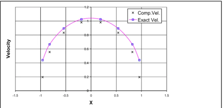
0 0.2 0.4 0.6 0.8 1 1.2
-1.5 -1 -0.5 0 0.5 1 1.5
X
Velocity
Comp.Vel.
Exact Vel.
Figure 5: Comparison of exact and computed values over the boundary of a circular cylinder for 16 linear boundary elements.
TABLE (2)
ELEMENT XM YM VELOCITY EXACT VELOCITY
1 -.99 .10 .98018E-01 .38677E+00
2 -.95 .29 .29029E+00 .46360E+00
3 -.88 .47 .47140E+00 .57934E+00
4 -.77 .63 .63439E+00 .70239E+00
5 -.63 .77 .77301E+00 .81490E+00
6 -.47 .88 .88192E+00 .90652E+00
7 -.29 .95 .95694E+00 .97082E+00
8 -.10 .99 .99518E+00 .10039E+01
9 .10 .99 .99518E+00 .10039E+01
10 .29 .95 .95694E+00 .97082E+00
11 .47 .88 .88192E+00 .90652E+00
12 .63 .77 .77301E+00 .81490E+00
13 .77 .63 .63439E+00 .70239E+00
14 .88 .47 .47140E+00 .57934E+00
15 .95 .29 .29028E+00 .46359E+00
16 .99 .10 .98017E-01 .38677E+00
17 .99 -.10 .98017E-01 .38677E+00
18 .95 -.29 .29028E+00 .46359E+00
19 .88 -.47 .47140E+00 .57934E+00
20 .77 -.63 .63439E+00 .70239E+00
21 .63 -.77 .77301E+00 .81490E+00
22 .47 -.88 .88192E+00 .90652E+00
23 .29 -.95 .95694E+00 .97082E+00
24 .10 -.99 .99518E+00 .10039E+01
25 -.10 -.99 .99518E+00 .10039E+01
26 -.29 -.95 .95694E+00 .97082E+00
27 -.47 -.88 .88192E+00 .90652E+00
28 -.63 -.77 .77301E+00 .81490E+00
29 -.77 -.63 .63439E+00 .70239E+00
30 -.88 -.47 .47140E+00 .57934E+00
31 -.95 -.29 .29029E+00 .46360E+00
32 -.99 -.10 .98017E-01 .38677E+00
TABLE (3)
ELEMENT XM YM VELOCITY EXACT VELOCITY
1 -1.00 .05 .49068E-01 .37355E+00
2 -.99 .15 .14673E+00 .39500E+00
3 -.97 .24 .24298E+00 .43401E+00
4 -.94 .34 .33689E+00 .48510E+00
5 -.90 .43 .42756E+00 .54321E+00
6 -.86 .51 .51410E+00 .60444E+00
7 -.80 .59 .59570E+00 .66590E+00
8 -.74 .67 .67156E+00 .72547E+00
9 -.67 .74 .74095E+00 .78155E+00
10 -.59 .80 .80321E+00 .83289E+00
11 -.51 .86 .85773E+00 .87852E+00
12 -.43 .90 .90399E+00 .91764E+00
13 -.34 .94 .94154E+00 .94964E+00
14 -.24 .97 .97003E+00 .97405E+00
15 -.15 .99 .98918E+00 .99051E+00
16 -.05 1.00 .99880E+00 .99880E+00
17 .05 1.00 .99880E+00 .99880E+00
18 .15 .99 .98918E+00 .99051E+00
19 .24 .97 .97003E+00 .97405E+00
20 .34 .94 .94154E+00 .94964E+00
21 .43 .90 .90399E+00 .91764E+00
22 .51 .86 .85773E+00 .87852E+00
23 .59 .80 .80321E+00 .83289E+00
24 .67 .74 .74095E+00 .78155E+00
25 .74 .67 .67156E+00 .72547E+00
26 .80 .59 .59570E+00 .66590E+00
27 .86 .51 .51410E+00 .60444E+00
28 .90 .43 .42756E+00 .54321E+00
29 .94 .34 .33689E+00 .48509E+00
30 .97 .24 .24298E+00 .43401E+00
31 .99 .15 .14673E+00 .39500E+00
32 1.00 .05 .49067E-01 .37355E+00
33 1.00 -.05 .49067E-01 .37355E+00
34 .99 -.15 .14673E+00 .39500E+00
35 .97 -.24 .24298E+00 .43401E+00
36 .94 -.34 .33689E+00 .48509E+00
37 .90 -.43 .42756E+00 .54321E+00
38 .86 -.51 .51410E+00 .60444E+00
39 .80 -.59 .59570E+00 .66590E+00
40 .74 -.67 .67156E+00 .72547E+00
41 .67 -.74 .74095E+00 .78155E+00
42 .59 -.80 .80321E+00 .83289E+00
43 .51 -.86 .85773E+00 .87852E+00
44 .43 -.90 .90399E+00 .91764E+00
45 .34 -.94 .94154E+00 .94964E+00
46 .24 -.97 .97003E+00 .97405E+00
47 .15 -.99 .98918E+00 .99051E+00
48 .05 -1.00 .99880E+00 .99880E+00
49 -.05 -1.00 .99880E+00 .99880E+00
50 -.15 -.99 .98918E+00 .99051E+00
51 -.24 -.97 .97003E+00 .97405E+00
52 -.34 -.94 .94154E+00 .94964E+00
53 -.43 -.90 .90399E+00 .91764E+00
54 -.51 -.86 .85773E+00 .87852E+00
55 -.59 -.80 .80321E+00 .83289E+00
56 -.67 -.74 .74095E+00 .78155E+00
57 -.74 -.67 .67156E+00 .72547E+00
58 -.80 -.59 .59570E+00 .66590E+00
59 -.86 -.51 .51410E+00 .60444E+00
60 -.90 -.43 .42756E+00 .54321E+00
61 -.94 -.34 .33689E+00 .48510E+00
62 -.97 -.24 .24298E+00 .43401E+00
63 -.99 -.15 .14673E+00 .39500E+00
64 -1.00 -.05 .49068E-01 .37355E+00
0 0.2 0.4 0.6 0.8 1 1.2
-1.5 -1 -0.5 0 0.5 1 1.5
X
Velocity
Comp.Vel.
Exact Vel.
Figure 6: Comparison of exact and computed values over the boundary of a circular cylinder for 32 linear boundary elements.
0 0.2 0.4 0.6 0.8 1 1.2
-1.5 -1 -0.5 0 0.5 1 1.5
X
Velocity
Comp.Vel Exact.Vel