Proceedings of the IASTED International Conference Parallel and Distributed Computing and Systems November 3-6, 1999, MIT, Boston, USA
Temperature Parallel Simulated Annealing with Adaptive Neighborhood for Continuous Optimization Problem
MITSUNORI MIKI,TOMOYUKI HIROYASU,MASAYUKI KASAI,MOTONORI IKEUCHI Department of Knowledge Engineering,
Doshisha University, Kyo-tanabe, Kyoto, 610-0321 Japan.
Email: [email protected]
Abstract
In this study, a temperature parallel simulated annealing with adaptive neighborhood (TPSA/AN) for continuous optimization problems is introduced. TPSA/AN is based on the temperature parallel simulated annealing (TPSA), which is suitable for parallel processing, and the SA that Corana developed for continuous optimization problems. The moves in TPSA/AN are adjusted to have equal acceptance rates. Because of this mechanism, the proposed method provides global search in the processors of parallel computers for high temperatures and local search in the processors for low temperatures in TPSA/AN. Therefore, all the processors are used for searching very efficiently. The TPSA/AN is evaluated for the standard test functions, and it is found that adopting the adaptive neighborhood range increases the searching ability of TPSA.
Key Words:Parallel Processing, Parallel Algorithms, Simulated Annealing, Temperature Parallel, Adaptive Method
1 Introduction
There is a strong incentive to parallelize the computation for optimization problems since it requires many iterations of analysis. Especially, new approaches to optimization problems such as genetic algorithms and simulated annealing, which are very effective for solving complicated optimization problems with many optima, require tremendous computational power.
Consequently, parallelization of these new optimization methods, which sometimes are called heuristic search methods[1], is very important.
It was Kirkpatrick et al. who first proposed simulated annealing, SA, as a method for solving combinatorial optimization problems[2]. It is reported that SA is very useful for several types of combinatorial optimization problems[3].
The advantages and the disadvantages of SA are well summarized in [4]. The most remarkable disadvantages are that
it needs a lot of time to find the optimum solution and it is very difficult to determine the proper cooling schedule. To determine the proper cooling schedule, many preparatory trials are needed.
When the cooling schedule is not proper, the guarantee of finding optimum solution is lost.
There are two approaches to shorten the calculation time in SA. One is determining the cooling schedule properly. SA with the proper cooling schedule can provide an optimum solution quickly. This approach is well reported by Ingber[4]. The other approach is to perform SA on parallel computers. Because of the rapid progress of parallel computers, there are several studies with this approach[5]. Among these studies, the temperature parallel simulated annealing (TPSA)[6], which was called the time-homogenous parallel annealing[7] before, is one of the algorithms that can overcome the cooling schedule problem. TPSA is an algorithm that can be carried out on parallel computers easily and does not require any cooling schedule. These are remarkable advantages. So far, TPSA has been applied to LSI allocation problems[6], travelling salesman problems[8], graph partition problems[7] and so on. However, there are very few studies that focus on continuous optimization problems. Therefore, the effectiveness of TPSA in continuous problems has not been clear.
In this study, a new TPSA approach that can be applied to continuous optimization problems is proposed. In the proposed approach, the SA that Corana developed and TPSA are combined and the neighborhood range is determined adaptively.
The approach is called temperature parallel simulated annealing with adaptive neighborhood (TPSA/AN).
2 Temperature Parallel Simulated Annealing
Comparing to sequential SA, there are more sophisticated algorithms that have proven that parallel probabilistic exchange of information gathered from processors annealing at constant but different temperatures can increase the overall rate of convergence. Kimura and Taki called this algorithm
temperature parallel simulated annealing (TPSA)[6]. In TPSA, each processor performs a sequential SA with a constant temperature for the whole annealing time, while the different temperatures are assigned to different processors. Two solutions in two processors with adjacent temperatures are exchanged with a certain probability at an interval of annealing time.
The important features of TPSA are as follows. (a) The cooling schedule is determined automatically because solutions decide their temperatures by themselves. (b) After getting solutions, when these solutions are not satisfied, TPSA can be restarted to get better solutions.
When the energy of solution at higher temperature is lower than that at lower temperature, the solutions are always exchanged. Otherwise, when the energy of solution at higher temperature is higher than that at lower temperature, the solutions are exchanged in accordance with the probability that is derived from the differences in temperature and energy. This probability function is defined in equation (1). By this method, the solutions that have low energy tend to concentrate to the lower temperature.
∆
−∆
<
∆
∆
= otherwise
T T
E T
E T if E
T E T pEX
' ) exp(
0 1
) ' , ' , , (
・
・
・ ( 1 )
where T is temperature, E is energy, and the prime means the state of the adjacent temperature. ΔT and ΔE are the differences in the temperature and the energy between two adjacent temperatures.
As mentioned before, in each processor of a parallel computer, one or several sequential SA with constant temperatures are performed. The acceptance probability is defined by the Metropolis standard that is shown in equation (2), where x is a design variable.
) ( ) (
) exp(
0 1
) ' , , (
old new
AC
E E
E
otherwise T
E
E E
E T p
x
x −
=
∆
−∆
≤
= ∆ ( 2 )
3 SA for continuous optimization problems
Simulated Annealing (SA)[2] has been proposed in the area of combinatorial optimization[3]. However, SA has been also used in the area of continuous optimization problems which had
a lot of local minima[4][9][10][11][12][13].
The definitions of the neighborhoods of solutions in the design space in SA are different between discrete and continuous optimization problems. For combinatorial optimization problems, the neighborhood of a solution is defined by a small change in the combination (e.g. 2-change neighborhood for the traveling salesman problems[14]). On the other hand, the neighborhood of a solution in continuous optimization problems is defined by a distance in the design space, which can be considered more easily than in combinatorial one.
Thus, for continuous optimization problems, it is important to determine the neighborhood range for generating a next point in a problem space[4]. If the neighborhood range is fixed to a constant range, the range should be determined individually for a particular problem. When the range is too large, it becomes difficult to get an accurate solution, while it takes much time to get better solution when the range is too small.
Therefore, for continuous optimization problems, there are several methods with adjustable neighborhood range. Many practitioners use novel techniques to narrow the range as the search progresses. For example, Boltzmann annealing method uses Gaussian distribution whose standard deviation is a squared root of the temperature[4]. Fast annealing method uses the Cauchy distribution[11]. In these methods, the neighborhood range is large if the temperature is high, while the neighborhood range is small if the temperature is low. However these methods are not effective for searching in problem spaces, because they do not use the information about objective functions.
There are several methods using the information about objective functions. Corana’s SA[10] uses the information, measured by a rate between accepted and rejected moves.
VFSR[9] uses the pseudo sensitivities of the objective function.
Dekker & Aarts’s SA[13] uses local search procedure (e.g.
steepest descent, quasi-Newton).
4 Temperature Parallel Simulated Annealing with Adaptive Neighborhood (TPSA/AN)
In this paper, we propose Temperature Parallel Simulated Annealing with Adaptive Neighborhood(TPSA/AN) which is the extension of TPSA by using the Corana’s SA[9] for continuous optimization problems. The difference between the conventional sequential SA for combinatorial optimization problems and TPSA/AN is that TPSA/AN has a procedure for exchanging solutions between different constant temperatures and a procedure for adjusting the neighborhood range. The
exchange of solutions and the adjustment the neighborhood range are executed at certain transitions.
In this algorithm, the distribution for generating a next point x’ from current point x is as follows:
rm x
x
i' =
i+
( 3 )where r is a random number generated in the range [-1, 1]; m is the neighborhood range. The algorithm in this paper has the same parameter m for each design values, while Corana’s SA has a different parameter for each design value. If the next point x’ lies outside the definition domain of an objective function, our algorithm will generate a new point again. The neighborhood range m is varied for adaptive search using equations (4), (5), (6) and (7):
) (p g m
mnew = old× ( 4 )
4 . 0
6 . 1 0
)
( = + p− c p
g , if p < 0.6 ( 5 )
1
4 . 0 4 . 1 0 ) (
−
+ −
= p
c p
g , if n < 0.4 ( 6 ) 1
) (p =
g , otherwise ( 7 ) where c is a multiplying factor for adjusting the neighborhood range ; p is a rate between accepted and rejected moves, and it is calculated from the following equation:
N n
p = /
( 8 )where N is a given number of transitions; n is the number of accepted moves in interval N. In this paper, parameter c is set to 2, following the Corana's paper.
In this algorithm, if the number of the accepted moves increases, the neighborhood range will be shortened adaptively by equations (4) and (5). If the number of the rejected moves increases, the neighborhood range will be stretched adaptively by equations (4) and (6). With this adaptation, the rate between the accepted and the rejected moves is adjusted to be in the range from 0.4 to 0.6, and this makes the computational effort on each parallel processor of a parallel computer effective.
5 Parallel Implementation
In TPSA/AN, inter-processor communications occur at the exchange of solutions in different processors at a certain annealing interval. Therefore, the communications are not frequent, and then TPSA/AN is very suitable for parallel
processing.
We use a PC-cluster with 8 processors, which are connected by the Fast Ethernet. PVM is used for a communication interface. The CPUs are Pentium II, 233MHz.
One temperature is assigned to one process in PVM.
Therefore, one process is running in one processor as the number of temperature stages is less than 8, but multiple processes are running in one processor as the number of temperature stages is greater than 9. In this study, 4 processes are running in one processor when the number of temperature stages is 32.
6 Minimization of Standard Test Function
To examine the performance of TPSA/AN, it is used for minimizing the standard test function, the Rastrigin function[14]. In this study, the function has two design variables. The function is expressed by equation (9). The optimum solution for the function exists at the origin and the values are 0.
The Rastrigin function has a relatively large area of local optima, and this kind of problems is appropriate for solving by genetic algorithms. However, it is considered that the performance of TPSA/AN can be evaluated well for such situations.
In this study, to evaluate the effectiveness of TPSA/AN, a sequential SA and TPSA are also implemented. The sequential SA and TPSA whose neighborhood ranges are fixed are called SA/F and TPSA/F, respectively. The sequential SA whose neighborhood range is changed adaptively is called SA/AN.
The parameters are summarized in Table 1 for the Rastrigin function with a maximum temperature (for the sequential SA, this means its starting temperature), a minimum temperature (for the sequential SA, this means its ending temperature), the number of annealing cycles, the Markov length, the cooling rate and the exchange intervals. The parameters are determined from the experience. The number of iterations in TPSA means the number of iterations in each temperature. Therefore, from the point of view for a single processor, the sequential SA performs annealing 32 times longer than in TPSA.
( )
− +
×
=
∑
= =
N
i
i i
N i
i N x x
x f
1 2 ,
1 ) ( 10) 10cos(2 )
( π ( 9 )
Table. 1 Parameters for the Rastrigin function
Algorithms SA TPSA
Number of Processes 1 32
Max. (Initial) temperature 10 10 Min. (final) temperature 0.01 0.01
Number of iterations 10240×32 10240 Markov Length 10240
Cooling rate 0.8
Exchange interval 32
7 Results of Numerical Experiments
TPSA/AN is carried out for the minimization of the Rastrigin function to discuss its effectiveness.
Figure 1 shows the energies obtained by SA and TPSA with respect to the neighborhood range. The neighborhood ranges are set to 0.01, 0.05, 0.l, 0.5, 1.0, 5.0 and the adaptive one. The interval used for adjusting the neighborhood range is 8. The results are shown as the average, best, and worst values of 10 trials. The relationship between the values of energy and the objective function is linear. Thus, the point that has the minimum value of the energy has the minimum value of the objective function, which is shown in equation (9).
Fig. 1 The performance of the various configuration for the Rastrigin function.
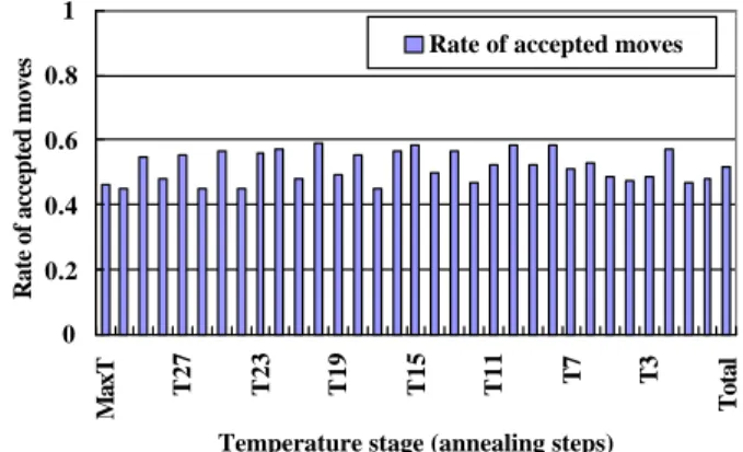
Figure 2 shows a history of the rate of the accepted moves in SA/AN. With the adjusting the neighborhood range, the rate is ranging from 0.4 to 0.6, as is expected. That is, the rate of the accepted moves maintains nearly constant during the search.
From Fig. 1, it is obvious that TPSA/AN is able to provide better solutions than SA/F, SA/AN and TPSA/F. Because the cooling schedule is not necessary to be determined in TPSA/AN, it can be said that TPSA/AN is a very powerful
algorithm for this type of optimization problems. In this study, the total number of annealing steps in SA and TPSA are fixed in order to find the clear differences are considered to appear.
0 0.2 0.4 0.6 0.8 1
MaxT T27 T23 T19 T15 T11 T7 T3 Total
Temperature stage (annealing steps)
Rate of accepted moves
Rate of accepted moves
Fig. 2 The history of the rate of the accepted moves in SA/AN From Fig. 1, it is clear that when the neighborhood range is fixed, SA/F has the minimum energy when the neighborhood range is 1.0, and TPSA/F has the minimum energy when the neighborhood range is 0.5. From these results, it is clear that the determination of the appropriate neighborhood range is very important to obtain good solutions. Also, it is recognized that the best values of the neighborhood ranges for SA/F and TPSA/F are different.
From Fig. 1, the performance of SA/F whose neighborhood range is properly fixed is better than that of TPSA/F with the best neighborhood range. This leads to that TPSA did not perform enough annealing in this case.
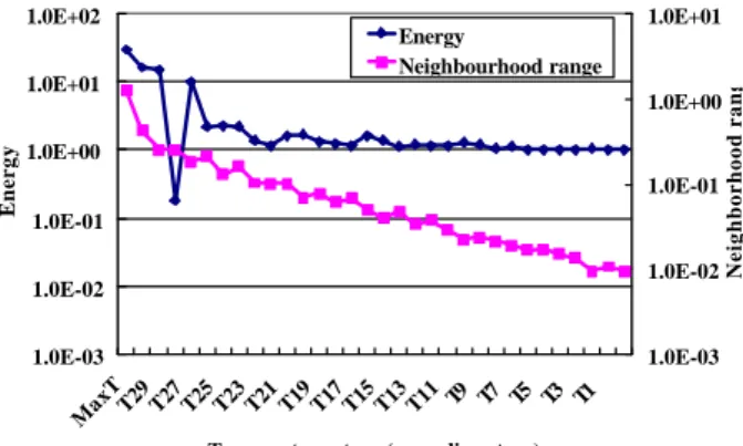
On the other hand, the quality of the solutions in SA/AN is worse than that of SA/F whose neighborhood range is properly fixed. The reason that the good solutions are not obtained is considered. In Fig. 3, the history of the energy and the neighborhood range in SA/AN are shown. From Fig. 3, it is found that the energy is not improved after the energy becomes 1.0. The point whose energy is 1.0 is the second optimum point.
Therefore, the solution is trapped at a local minimum in SA/AN.
From Fig. 3, it is also found that the neighborhood range of SA/AN is decreasing. This means that the solution is trapped in a local minimum and the acceptance rate becomes small. Then the neighborhood range becomes small to increase the acceptant rate. By this mechanism, the solution can not escape from the local minimum. Thus, adjusting the neighborhood range has a role of convergence acceleration. In this case, the solutions are converged to a local optimum.
1.0E-07 1.0E-05 1.0E-03 1.0E-01 1.0E+01 1.0E+03
AN 5 1 0.5 0.1 0.05 0.01
Neighborhood range
Energy
SA_Best SA_Ave.
SA_Worst TPSA_Best TPSA_Ave.
TPSA_Worst
1.0E-03 1.0E-02 1.0E-01 1.0E+00 1.0E+01 1.0E+02
MaxTT29 T27 T25 T23 T21 T19 T17 T15 T13 T11 T9 T7 T5 T3 T1 Temperature stage (annealing steps)
Energy
1.0E-03 1.0E-02 1.0E-01 1.0E+00 1.0E+01
Neighborhood range
Energy
Neighbourhood range
Fig. 3 The history of the Energy and the neighborhood range on SA/AN.
On the other hand, because TPSA/AN provides good solutions, adjusting the neighborhood range does not accelerate the convergence of the solutions to a local optimum. This is ascertained from the results in Figs. 4 and 5. In Fig. 4, the histories of the temperature and neighborhood range of the best solution are shown. The history of the energy of the best solution is also shown in Fig. 5.
From Fig. 4, it is found that the temperature scheduling is determined automatically in TPSA/AN, and it is also found that the neighborhood range is also changed with respect to the steps and this change is related to the change of the temperature and the landscape of the objective function. From Figs. 4 and 5, it can be said that there are two aspects in these histories. One is the acceleration of the convergence to a local optimum and the other is escaping from a local optimum. The latter mechanism is the reason that TPSA/AN can provide good solutions.
As mentioned before, the acceleration of convergence comes from the mechanism of the adjustment of the neighborhood range. The escaping from a local optimum comes from the effect of a global search at high temperature stages. Because of the acceleration of convergence and the escaping from a local optimum, TPSA/AN can find the good solutions with 1/32 of the annealing steps of the sequential SA.
Figure 6 shows the calculation time of TPSA/AN that provides optimum solutions for the Rastrigin function with 8 CPUs and 32 temperature processes. From this figure, it is found that the calculation time is reduced to about 55% by parallel processing and the parallel efficiency is about 30% in this case. This parallel efficiency is not good for 8 CPUs. On the other hand, in the study of Konishi and Taki[8], the parallel efficiency of TPSA that is implemented for combinatorial optimization problems with 32 CPUs reached the parallel efficiency of almost 100 %. The reason for the low parallel
efficiency in this study is the simplicity of the test functions used in this study. The function is a simple numerical function with only 2 design variables, and the calculation load for these functions are very small, and the granularity of parallel processing becomes very small.
1.00E-03 1.00E-02 1.00E-01 1.00E+00 1.00E+01
0 2000 4000 6000 8000 10000 12000
Annealing steps
Neighborhood range
1.00E-02 1.00E-01 1.00E+00 1.00E+01
Temperature
Neighborhood range Temperature
Fig. 4 The history of the temperature and neighborhood range on TPSA/AN
1.00E-06 1.00E-04 1.00E-02 1.00E+00 1.00E+02
0 2000 4000 6000 8000 1 0 0 0 0 1 2 0 0 0 Annealing steps
Energy
Fig. 5 The history of the energy on TPSA/AN
0 . 0 1 . 0 2 . 0 3 . 0 4 . 0
S A / A N T P S A / A N Algorithm types
Calculation time (sec)
Fig. 6 The comparison of the calculation times of TPSA with sequencial SA.
8 Conclusions
In this study, the temperature parallel simulated annealing with adaptive neighborhood (TPSA/AN) that is able to solve optimization problems whose design variables are continuous is proposed. The effectiveness of TPSA/AN is investigated through the Rastrigin function. The following results are derived in this study.
1)The neighborhood range affects the search abilities of SA and TPSA in continuous optimization problems.
Therefore, the determination of the best neighborhood is very important.
2)The optimum obtained by TPSA/F with the best neighborhood range is worse than the one obtained by SA/F with the best neighborhood range.
3)The optimum solution obtained by TPSA/AN is better than the one obtained by SA/F, SA/AN and TPSA/F.
4)TPSA/AN has high ability of global searching and quick convergence to the global optimum. Therefore, TPSA/AN is a powerful algorithm for continuous optimization problems.
Reference
[1]Beasley, J., Dowsland, K., Glover, F., Laguna, M., Peterson, C., Reeves, C. R. and Söderberg, B., Modern Heuristic Techniques for Combinatorial Problems, Blackwell Scientific Publications, 1993
[2]Kirkpatrick, S., Gelett Jr. C. D., and Vecchi, M. P., Optimization by Simulated Annealing, Science, 220(4598), 1983, 671-680
[3]Aarts, E. and Korst, J., Simulated Annealing and Boltzmann Machines, John Wiley & Sons, 1989
[4]Ingber, L., Simulated Annealing: Practice versus Theory, J.
of Mathl. Comput. And Modelling, 18(11), 1993, 29-57 [5]Holmqvist, K., Migdalas, A., and Pardalos, P. M.,
Parallelized Heuristics for Combinatorial Search, in Parallel Computing in Optimization, Migdalas, A. et al.
eds., Kluwar Academic Publishers, 1997, 269
[6] Konishi, K., Taki, K. and Kimura, K., Temperature Parallel Simulated Annealing Algorithm and Its Evaluation, Trans. on Information Processing Society of Japan, 36(4), 1995, 797-807 (in Japanese)
[7] Kimura, K. and Taki, K., Time-homogeneous Parallel Annealing Algorithm, The 13th IMACS World Congress of Computation and Applied Mathematics, 1991
[8] Konishi, K., Yashki, M. and Taki, K., An Application of Temperature Parallel Simulated Annealing to the
Traveling Salesman Problem and its Efficient Implementation on the Distributed Memory Parallel Machine, 1996 Joint Symposium of Parallel Processing, 1996, 153-160 (in Japanese)
[9]Ingber, L., Genetic Algorithms and Very Fast Simulated Reannealing: A Comparison, Mathematical and Computer Modeling, 16(11), 1992, 87-100
[10]Corana, A., Marhesi, M., Martini, C. and Ridella, S., Minimizing Multimodal Functions of Continuous Variables with the “Simulated Annealing” Algorithm, ACM Trans. on Mathematical Software, 13(3), 1987, 262- 280
[11]Szu, H. and Hartley, R., Fast Simulated Annealing, Physics Letters A, 122(3,4), 1987, 157-162
[12]Rosen, B., Functional Optimization based on Advanced Simulated Annealing, IEEE Workshop on Physics and Computation, PhysComp92 (Dallas, Texas), 1992, 289- 293
[13]Dekkers, A. and Aarts, E., Global optimization and simulated annealing, Mathematical Programming, 50, 1991, 367-393
[14]p.7 of the reference [4]
[15]Whitley, D., Mathias, K., Rana, S. and Dzubera, J., Evaluating Evolutionary Algorithms, Artificial Intelligence, 85, 1996, 245-2761