Growing Ant Colony Optimization with Intelligent and Dull Ants
and its Application to TSP
Sho Shimomura
Dept. Electrical and Electronic Eng., Tokushima University
Email:[email protected]
Haruna Matsushita
Dept. Reliability-based Information Systems Eng., Kagawa University
Email:[email protected]
Yoko Uwate
Dept. Electrical and Electronic Eng., Tokushima University
Email: [email protected]
Yoshifumi Nishio
Dept. Electrical and Electronic Eng., Tokushima University
Email: [email protected]
Abstract— This study proposes an Growing Ant Colony Op- timization with Intelligent and Dull Ants (GIDACO). In the GIDACO algorithm, two kinds of ants coexist: intelligent ants and dull ants. In addition, the number of ants in the colony is increased with the passage of time. The new ant is added based on the best ant which has the best tour. Also, the added ant is decided whether the dull ant or intelligent ant by the probability.
By growing the colony, the structure of GIDACO is changed flexibly and automatically depending on the problem. Moreover, the growing can also reduce the simulation time because the simulation time depends on the number of ants. We apply GIDACO to Traveling Salesman Problems (TSPs) and confirm that GIDACO obtains more effective results than the standard ACO which consists of only the intelligent ants.
I. INTRODUCTION
Ant Colony Optimization (ACO) [1][2] is proposed to solve difficult combinatorial optimization problems, such as Travel- ing Salesman Problem (TSP), graph coloring problem, routing in communications networks, Quadratic Assignment Problem (QAP) [3]-[7] and so on. TSP is a problem in combinatorial optimization studied in an operations research and a theoretical computer science. In TSP, given a list of cities and their pairwise distances, the task is to find the shortest possible tour that each city exactly visited once. In the ACO algorithm, multiple solutions called “ants” coexist, and the ants drop a substance called the pheromone. Pheromone trails are updated depending on the behavior of the ants. By communicating with other ants according to the pheromone strength, the algorithm tries to find the optimal solution. However, ACO has a problem which is to trap at local solutions. Therefore, it is important to enhance the algorithm performances by improving its flexibility.
Meanwhile, it has been reported that about 20 percent of the ants are unnecessary ants called “dull ant” in the real ant’s world [8]. The dull ant keeps dawdle its colony whereas the other ants in the colony perform feeding behavior. In
a computational experiment, the researchers performed the feeding behavior by using intelligent ants, which can trail the pheromone exactly, and dull ants which cannot trail the pheromone. From these results, the ants group including the dull ants can obtain more foods than the group containing only the intelligent ants. The dull ants are regarded as having task which find the new food sources by dawdle. It means that the coexistence of the intelligent and dull ant improves the effectiveness of the feeding behavior.
In this study, we propose a new type of the ACO algorithm called Growing Ant Colony Optimization with Intelligent and Dull Ants (GIDACO). The first important feature is that two kinds of ants coexist. The one is an intelligent ant and the another is a dull ant. The intelligent ant can trail the pheromone and the dull ants cannot trail the pheromone. The second important feature of GIDACO is that the number of ants in the colony is increased with the passage of time. In other words, there are a few ants in the initial colony, however, the colony grows depending on ants’ conditions. The new ants are added based on the ant which obtained the best tour.
Also, the added ant is decided whether dull ant or intelligent ant by the probability. By growing the colony, the structure of GIDACO is changed flexibly and automatically depending on the problem. Moreover, the growing can also reduce the simulation time because the simulation time depends on the number of ants. Because their features are essentially similar to the real ant’s world, we can say that GIDACO algorithm is nearer to the real ant colony than the standard ACO algorithm.
This paper is organized as follows. The basic method of ACO is introduced in the Section II. We explain the GIDACO algorithm in detail in the Section III. In the Section IV, we apply GIDACO to four kinds of TSPs whose number of cities are different. Furthermore, we investigate the behavior of GI- DACO in detail. Performances are evaluated quantitatively in comparison with the standard ACO. We confirm that GIDACO
- 44 -
IEEE Workshop on Nonlinear Circuit Networks December 9-10, 2011
Initialize deposited pheromone Start
No
M ants are set to city at random. k = 1
Update pheromone Yes
τ0
pij Choose the next city j according to the choice probability
All ants visited all cities Ant k visited all cities
Yes k= k+ 1 No
No
End Yes
Update pheromone
tmax
t<
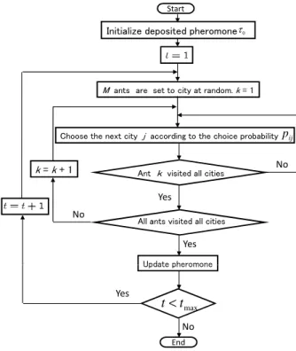
Fig. 1. Flowchart of the ACO algorithm.
can obtain a more effective results than the standard ACO.
Finally, the Section V concludes this paper.
II. THE BASIC ALGORITHM OFACO
ACO is popular search algorithms and applied to various applications. In this section, we introduce the basic algorithm of ACO.
A flowchart of the ACO algorithm is shown in Fig.1.N- city of TSP is denoted as
S≡ {P1, P2,· · ·, PN}, Pi≡(xi, yi), (1) where the data area is normalized from 0 to 1, andPi denotes the i-th city position (i= 1,2,· · ·, N). Each antk(totalM) is deposited on a city selected at random.
[ACO1](Initialization): Let the iteration numbert= 0.τij(t) is the amount of pheromone deposited on the path (i, j) between the cityiandj at timet, andτij(t)is initially set to τ0.
[ACO2](Find tour): The visiting city is chosen by according to the probability pij(t)as shown in Fig. 2. The probability of k-th ant moving from the cityi toj is decided by
pkij(t) = [τij(t)]α[ηij]β
Σl∈Nk[τil(t)]α[ηil]β, (2) where k = 1,2,· · ·, M, and 1/ηij is the distance of the path (i, j). The adjustable parameters α and β control the weight of the pheromone intensity and of the city information, respectively. Therefore, the searching ability goes up and down by changingαandβ. As Eq. (2), the ants judge next city by
City i
City 3 City 2
City 1
( )
tpi1
( )
tpi2 pi3
( )
tFig. 2. Probabilitypij(t)of ants. The visiting city is chosen by probability pij(t).
both the pheromone and the distance from the present location.
Nk is a set of the cities that k-th ant has never visited. The ants repeat choosing next city until all the cities are visited.
[ACO3](Pheromone update): After all ants have completed their tours, the amount of pheromone deposited on each path is updated. The tour lengthLk(t)is computed, and the amount of pheromone∆τkij(t)deposited on the path(i, j)byk-th ant is decided as
∆τkij(t) =
{ 10/Lk, if (i, j)∈Tk(t)
0, otherwise, (3)
whereTk(t)is the tour obtained byk-th ant, andLk(t)is its length. Total amount of pheromone τij(t)of each path (i, j) is updated depending on ∆τkij(t);
τij(t+ 1) = (1−ρ)τij(t) +
∑M
k=1
∆τkij(t), (4) whereρ∈[0,1]is the rate of pheromone evaporation.
[ACO4] Let t=t+ 1. Go back to [ACO2] and repeat until t=tmax.
III. GROWINGANTCOLONYOPTIMIZATION WITHINTELLIGENT ANDDULLANTS
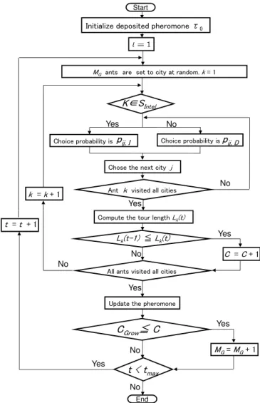
We explain the proposed GIDACO algorithm in detail. A flowchart of the GIDACO algorithm is shown in Fig. 3. The first important feature of GIDACO is that two kinds of ants coexist; intelligent ant which can exactly trail the pheromone and dull ant which cannot trail the pheromone for making the tour. The second important feature of GIDACO is that the number of ants is increased with the passage of time. In other words, the colony grows depending on the problem. N-city positions of TSP is set to according to Eq. (1). First, each ant k (totalMG) is deposited on a city selected at random. Ants are classified into a set of the intelligent ants SIntel, namely, the initial colony consists of only the intelligent ants.
[GIDACO1](Initialization): Let iteration number t = 0 and initialize the pheromone τij(t)according to [ACO1].
[GIDACO2](Find tour): For the intelligent ants and the dull ants, the visiting city is chosen by the probability pij,I(t)and
- 45 -
Initialize deposited pheromone τ0 Start
MGants are set to city at random. k= 1
No Yes
Choice probability is Choice probability is
Chose the next city j
Ant k visited all cities Yes
No k = k+ 1
K∈SIntel
pij, I pij, D
No
No End Yes
Update the pheromone Yes All ants visited all cities Compute the tour length Lk(t)
Yes
No
CGrow≦ C
t < tmax
t = t + 1
Lk(t-1) ≦ Lk(t) No
Yes C = C+ 1
MG= MG+ 1
Fig. 3. Flowchart of the GIDACO algorithm.
pij,D(t)as shown in Fig. 4. The probability ofk-th ant moving from the cityi toj is decided by
pkij,D(t) = [ηij]βD
Σl∈Nk[ηil]βD, if k∈Sdull (5)
pkij,I(t) = [τij(t)]α[ηij]βI
Σl∈Nk[τil(t)]α[ηil]βI. otherwise, (6) The adjustable parameters βI and βD control the weight of the city information of the intelligent ant and of the dull ant, respectively. As Eq. (5) does not include the amount of deposited pheromone τij(t) and τil(t), the dull ants cannot trail the pheromone. The dull ants judge next city depending on only the distance from the present location, in contrast to the intelligent ants which judge next city by the pheromone and the distance from the present location.
[GIDACO3](Pheromone update): After all ants have com- pleted their tours, the amount of deposited pheromone on each path is updated. We should note that the dull ants can deposit the pheromone on the path, though, they cannot trail
City i
City 3 City 2
City 1 ( )t
pi1,I
( )t
pi2,I pi3,I( )t ( )t
pi1,D
( )t
pi2,D
( )t
pi3,D
Intelligent ant Dull ant
Fig. 4. Probabilitypij(t)of Intelligent and Dull ants.The visiting city of intelligent ant is chosen by the probabilitypij,I(t). The visiting city of dull ant is chosen by the probabilitypij,D(t)which does not include the amount of pheromone.
the pheromone. Then, the tour length Lk(t) is computed for both the intelligent and dull ants, and the amount of pheromone∆τkij(t)deposited byk-th ant on the path (i, j) is decided according to Eq. (3), Updateτij(t)of each path (i, j) according to Eq. (4)
[GIDACO4](Growing): After the their tour length Lk(t) is computed, we evaluate the tour length Lk(t) and consider whether the colony should be grown. A growing rule is as follows;
C=
{ C+ 1, if Lk(t−1)≤Lk(t)
C, otherwise, (7)
where C is a counter which counts the number of times which obtained results are worse than that of last iteration.
The number of ants is decided by MG=
{ MG+ 1 andC= 0, if C≥CGrow
MG. otherwise, (8)
The adjustable parameter CGrow controls the rate of ants in- crease. The added ant is decided whether dull ant or intelligent ant by the probability. The dull ant is added by according to the probability Pm, in contrast the intelligent ant is added by the probability(1−Pm). In addition, the added ant is affected by the best ant. Namely, the new ant is deposited in the same city of ant which obtained best tour.
[GIDACO5] Lett=t+1. Go back to [GIDACO2] and repeat until t=tmax.
IV. NUMERICALEXPERIMENTS OFTSP
In order to evaluate a performance of GIDACO and to investigate its behavior, we apply GIDACO to various TSPs.
We compare GIDACO with the standard ACO.
In the experiments, the number of ants M in the standard ACO is set to the same as the number of cities, namely M = N. However, the initial number of ants MG in the GIDACO is set to the one-tenth of the number of cities, namely MG=N/10. Therefore, the number of antsMG in GIDACO is changed from N/10 to N. The standard ACO contains ants whose choice probability is decided by Eq. (2). GIDACO includes dull ants and intelligent ants whose choice probability
- 46 -
TABLE I
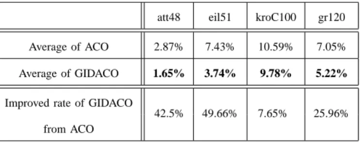
RESULTS OF THE STANDARDACOANDGIDACO.
att48 eil51 kroC100 gr120 Average of ACO 2.87% 7.43% 10.59% 7.05%
Average of GIDACO 1.65% 3.74% 9.78% 5.22%
Improved rate of GIDACO
42.5% 49.66% 7.65% 25.96%
from ACO
is decided by Eq. (6). We repeat the simulation 20 times for all the problems. The parameters of two methods are set as follows;
τ0= 10, ρ= 0.3, α= 1, β=βI =βD= 5, Pm= 0.2, CGrow= 30, tmax= 2000,
where the evaporation rateρ, the weight of pheromoneα, the weight of distanceβ,βI andβD, probability of dull ant Pm, the rate of ants increaseCGrow and the search limitt=tmax are fixed values. In order to compare obtained solutions with the optimal solution, we use an error rate as follow;
Error rate[%]
=(obtained solution)−(optimal solution) (optimal solution) ×100.
(9)
This equation shows how close to the optimal solution the ACOs obtain the tour length. Thus, the error rate nearer 0 is more desirable. Furthermore, in order to evaluate how well the solution of GIDACO are improved from that of ACO, we use an improved rate as follow;
Improved rate[%] =
(Avg.of Error of ACO)−(Avg.of Error of GIDACO) (Avg.of Error of ACO) ×100.
(10) The TSPs are conducted on att48 (composed of 48 cities), eil51 (composed of 51 cities), kroC100 (composed of 100 cities) and gr120 (composed of 120 cities). These problems are quoted from TSPLIB [9]. The simulation results of the standard ACO and GIDACO are shown in TableI.
In this table, the average values nearer 0 are more desirable.
We can confirm that the proposed GIDACO obtained the best results than the standard ACO for all the problems. Further- more, we investigate the relationship between the performance and the number of ants of GIDACO for eil51. Figure 5 shows the simulated result for 1 trial. We can see that obtained solutions are improved by increasing the number of ants.
Also, GIDACO can reduce the simulation time because the simulation time depends on the number of ants. From these results, we can say that GIDACO is more effective algorithm than the standard ACO in solving TSPs.
0 50 100 150 200 250 300 350 400 450 500
0 20 40 60
Iteration
The number of ants
0 50 100 150 200 250 300 350 400 450 500450
500 550 600
Tour length
The total number of ants The number of intelligent ants The number of dull ants Minimum
Fig. 5. Relationship between the performance and the number of ants in the simulation of eil51.
V. CONCLUSION
In this study, we have proposed Growing Ant Colony Optimization with Intelligent and Dull Ants (GIDACO). We have investigated the performances of GIDACO by applying it to four TSPs. We have confirmed that GIDACO including the dull ants obtained better results than the standard ACO which containing only the intelligent ants. We considered that the structure of GIDACO which changed flexibly and automatically depending on the problem is effective. From these results, we can say that GIDACO is more effective algorithm than the standard ACO in solving TSPs.
REFERENCES
[1] M. Dorigo and T. Stutzle, Ant Colony Optimization, Bradford Books, 2004.
[2] M. Dorigo, V. Maniezzo and A. Colorni, “Ant System: Optimization by a Colony of Cooperating Agents,” IEEE Trans. Systems, Man, and Cybernetics, Part B: Cybernetic, vol.26 no. 1, pp. 29-41, 1996.
[3] M. Dorigo and L. M. Gambardella, “Ant Colonies for the Traveling Salesman Problem,” BioSystems, vol. 43, pp. 73–81, 1997.
[4] M. Dorigo, G. D. Caro and L. M. Gambardella, “Ant Algorithms for Discrete Optimization,” Artificial Life vol. 5 no. 2, pp. 137-172, 1999.
[5] Blum and Merkel (eds.), Swarm Intelligence, Springer, 2008.
[6] Inspiration for optimization from social insect behavior. E. Bonabeau, M.
Dorigo and G. Theraulaz.
[7] V. Maniezzo and A.Colorni, “The ant system applied to the quadratic assignment problem,” IEEE Transactions on Knowledge and Data Engi- neering vol. 11 no. 5, pp. 769-778, 1999.
[8] H. Hasegawa, “Optimization of GROUP Behavior,” Japan Ethological Society Newsletter, no. 43, pp. 22-23, 2004 (in Japanese).
[9] G. Reinelt, “TSPLIB-A traveling salesman problem library, ” ORSA J.
Comput. Vol. 3: pp.376-384, 1991.