Characterizations of Graphs for Eﬃcient Algorithms

(1)

有限群を用いた計算困難なグラフ問題の緩和と，効率的アルゴリズムのためのグラフの特徴づけ

西山, 宏

http://hdl.handle.net/2324/2236254

出版情報：Kyushu University, 2018, 博士（工学）, 課程博士バージョン：

権利関係：

(2)

Characterizations of Graphs for Eﬃcient Algorithms

Hiroshi Nishiyama

(3)

(4)

Abstract

It was 1971 when the notion of NP-completeness was introduced by Cook. Karp proposed 21 NP-complete problems, and more than half of them are graph problems, including Hamiltonian cycle problem, vertex cover, and chromatic number. These hard problems, however, are solved eﬃciently when input graphs have specific structures.

Understanding graph structures is an important and prospective approach for designing eﬃcient graph algorithms.

Relaxation of a problem is a standard strategy to attack hard problems; consider a relaxed variant of a hard problem, find good characterizations for it, and apply the idea of the characterizations to the original hard problem. Motivated by the development of new technologies for relaxation, this paper focuses on relaxations using finite groups.

The target of relaxation is not unique; relaxation of the constraints of a problem, relaxation of “for any input” condition (restricting the class of inputs), relaxation of objective function (approximation), and so on. To begin with, this thesis considers a variant of the Hamiltonian cycle problem by relaxing the constraint. We give rise to a new problem,parity Hamiltonian cycle, which is a relaxed variant of the Hamiltonian cy- cle problem. A parity Hamiltonian cycle is a closed walk (possibly using each edge more than once) which visits every vertex an odd number of times. We are concerned with the problem in both undirected graphs and directed graphs. We give some good characterizations for both undirected graphs and directed graphs which have parity Hamiltonian cycles. Based on the characterizations, we present eﬃcient algorithms for both problems.

Particularly, the existence of a parity Hamiltonian cycle in a directed graph is characterized by a linear system over GF(2), thus the problem is solved by solving the linear system. Next we consider the Hamiltonian cycle problem for covering graphs, which are defined by finite groups. Batagelj et al. (1982) showed a very simple characterization of the Hamiltonicity of the Cartesian product of a tree and a cycle which is represented as a covering graph. We show the same characterization as Batagelj et al.’s is applicable for two larger graph classes.

Finding a spanning tree of minimum weight with bounded diameter is known to be NP-hard. We give rise to a variant of the problem, the odd depth tree problem. An odd depth tree is a rooted spanning tree such that the distance of each leaf and the root is odd. We show the NP-hardness for non-bipartite graphs, while we present a complete

(5)

characterization for bipartite graphs. We also consider the problem for directed graphs, and show similar characterizations and complexity results to the undirected case.

(6)

Acknowledgment

First of all the author is very grateful to my supervisor Shuji Kijima. He helped me a lot and gave me advice about my research, presentations, thesis and paperworks. I was on half-way to giving up the Ph. D. course, but he patiently waited for me while I was taking a year oﬀ, and when I was back he encouraged me to finish this great work up.

Without his eﬀort I could not hang tough to work on this thesis.

I would like to express my sincere gratitude to my ex-supervisor Masafumi Yamashita who kindly gave me advice during my undergraduate and master courses, and the first two years of my Ph. D. course. I also would like to appreciate the associated professor Yukiko Yamauchi for taking great care of me and giving advice about my research.

I am grateful to the professor Eiji Takimoto and the associate professor Naoyuki Kamiyama who cooperatively discussed my research and gave me a lot of helpful advice.

I would like to thank every my current members and ex-colleagues in my laboratory who I have met in the seven years of my life here. I appreciate their kindness which helped me a lot. I have grown in my mind in many aspects throughout the relationship with them.

Finally, I appreciate my family, especially my mother Junko for her economic and mental assistance.

(7)

(8)

Chapter 1 Introduction

It was 1971 when Stephen A. Cook posed the notion of NP-completeness, and Leonid Levin independently found essentially the same notion around the same time. Since then, the conjecture P ̸= NP has been a major open problem in the theoretical com- puter science. Graph algorithms have been the central issue in the context. In 1972, Richard R. Karp presented 21 NP-complete problems, in which more than half of them are problems on graphs such as Hamiltonian cycle (HC), vertex cover, chromatic number, etc. However, those hard problems are easily solved for some graphs; the Hamil- tonian cycle problem is polynomial time solvable for strongly connected path-mergeable graphs, locally semi-complete graphs [3], cocomparability graphs [17], distance heredi- tary graphs [32], etc. Understanding graph structures is an important and prospective approach for designing eﬃcient graph algorithms. Then, the ultimate goal of this study in future is to find good characterizations for any problems in NP.

As an approach, it may be a natural idea to begin with considering arelaxed variant, of a hard problem, finding good characterizations of it, and applying the idea of the characterizations to the original hard problem. Relaxation is a standard approach to attack a hard problem. The traveling salesman problem (TSP) in a graph, is regarded as a relaxed version of the HC problem, in the sense that the condition of visiting number on each vertex is relaxed to more than once. Another example may be a two-factor (in cubic graphs), which relaxes the condition of the connectivity of an HC, but a two-factor must contain each vertex exactly once (cf. [29, 30, 8, 9]). Motivated by a development of new techniques for relaxation, this paper focuses on relaxations using finite groups. In the areas of graph theory and matroid theory, group-labeled graphs recently attract lots of attension, and are intensively investigated [14, 38, 39, 54]. Theparity is regarded as a cyclic group of order two. Graph problems with parity constraints have been well studied;

realizing plane graphs with prescribed parity of degrees of vertices [1], strong connected orienting of undirected graphs with parity constraints for degrees [22], edge-coloring with parity constraint [12], subset feedback set problem with parity condition [35], multi-way cut with parity constraint [44], etc.

(12)

The target of relaxation is not unique; relaxation of the constraints of a problem, relaxation of “for any input” condition (restricting the class of inputs), relaxation of objective function (approximation), and so on. In this thesis, we consider a variant of Hamiltonian cycle problem by relaxing the constraint of the Hamiltonian cycle problem.

First we introducethe parity Hamiltonian cycle problem(PHC), which is a relaxed variant of the Hamiltonian cycle problem. A PHC is a closed walk (possibly using each edge more than once) which visits every vertex an odd number of times. We are concerned with the problem in both undirected graphs and directed graphs. Particularly, a characterization of directed graphs is given by a GF(2) linear system and the problem is easily solved using the linear system. Next we consider the Hamiltonian cycle problem restricting the class of input graphs. The HC problem for graphs possessing some symmetry such as vertex-transitive graphs is a major target in graph theory. This thesis is concerned with covering graphs, which are defined by finite groups, and gives a new characterization of Hamiltonicity. Also we will be concerned with another NP-hard problem. A spanning tree is a connected acyclic subgraph. While a spanning tree in a graph is easily found, finding the one with bounded diameter is known to be NP-hard. In this thesis we consider the odd depth tree problem, a variant of the above problem relaxing the constraint using parity.

1.1 Relaxation of Constraints: Parity Hamiltonian Cycle Prob- lem

1.1.1 Undirected PHC Problem

A Hamiltonian cycle (HC) is a cycle which visits every vertex exactly once. The question if a given graph has a Hamiltonian cycle is a celebrated NP-complete problem due to Karp [36]. It could be a natural idea for the HC problem to relax the condition on the visiting number. The traveling salesman problem (TSP) is a celebrated optimization problem to minimize the length of a walk, where the walk must visit every vertex at least once, while an HC visits every vertex exactly once. This thesis proposes another relaxation of the HC problem using parity. The parity Hamiltonian cycle (PHC), which is a variant of the Hamiltonian cycle: a PHC is a closed walk which visits every vertex an odd number of times (see Section 2.1, for more rigorous description). Note that a closed walk is allowed to use an edge more than once. The PHC problem is to decide if a given graph has a PHC. We remark that if the condition “odd number of times” is changed to

“even number of times,” the problem becomes trivial: just finding a spanning tree and tracing it twice suﬃces.

It may not be trivial if the PHC problem is in NP, since the length of a PHC is unbounded in the problem. In Section 2.3 we show that the PHC problem is in P, in fact. Precisely, we give a complete characterization of the graphs which have PHC’s.

(13)

Table: 1.1: Time complexity of the PHC problem.

Each edge is used at most z times Complexity Refinement

z ≥4 P (Thm. 2.7)

z = 3 NP-complete (Thm. 2.10) ⇒ Table 1.2

z = 2 NP-complete (Thm. 2.10)

z = 1 NP-complete (Thm. 2.9)

Table: 1.2: Time complexity of the PHC₃ problem.

Edge connectivity Complexity Refinement by graph classes 4-edge-connected P (Thm. 2.11)

3-edge-connected unknown P forP₆-free or C_≥₅-free 2-edge-connected NP-complete (Thm. 2.10) (Section 2.5) 1-edge-connected NP-complete P forP₆-free or C_≥₅-free

(from 2-edge-connected case) (Section 2.6.1)

Furthermore, we show that if a graph has a PHC then we can find a PHC₄ in linear time, where PHC_z for a positive integerz denotes a PHC which uses each edge at mostz times.

In contrast, Section 2.4 shows that the PHCz problem is NP-complete for eachz = 1,2,3 (see Table 1.1)¹. We then further investigate the PHC₃ problem. In precise, the PHC₃ problem is NP-complete for two-edge-connected graphs, while Section 2.4.1 shows that it is solved in polynomial time for four-edge-connected graphs. The complexity of the PHC₃ for three-edge-connected graphs remains unsettled (see Table 1.2).

As an approach to the PHC₃ problem for three-edge-connected graphs, we in Sec- tion 2.5 utilize the celebrated ear-decomposition, which is actually a well-known charac- terization oftwo-edge-connected graphs. Then, Section 2.5 shows that the PHC₃problem is in P for any two-edge-connected C_≥₅-free or P₆-free graphs (see Section 2.2 for the graph classes). The classes ofC_≥₅-free andP₆-free contain some important graph classes such as chordal, chordal bipartite and cograph. We remark that it is known that the Hamiltonian cycle is NP-complete forC_≥₄-free graphs, as well asP₅-free graphs (cf. [10]).

In precise, we in Section 2.5 introduce a stronger notion ofall-roundness (andbipar- tite all-roundness) of a graph, which is a suﬃcient condition that a graph has a PHC.

Catlin [13] presented a similar notion of collapsible in the context of spanning Eulerian subgraphs, and the all-roundness is an extended notion of collapsible. Then, we show that any two-edge-connected C_≥₅-free and P₆-free graphs are all-round or bipartite all-

1Notice that those hardness results are independent, e.g., “z = 3 is hard” does not imply “z= 2 is hard,” and vice versa.

(14)

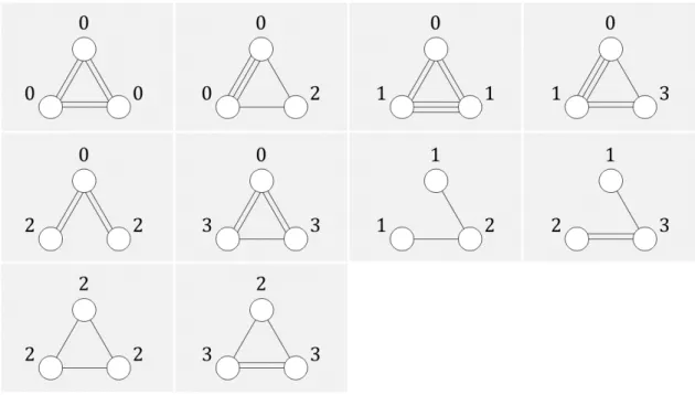
Figure: 1.1: PHC3 is in P for C_≥5-free graphs and P6-free graphs.

round. We conjecture that any two-edge-connected C_≥₇-free graphs are all-round, while it seems not true for C_≥₈-free nor P₇-free.

Section 2.6 is for miscellaneous discussions. Section 2.6.1 shows that the PHC₃ problem is in P for any C_≥5-free or P6-free graphs, and extends the results in Section 2.5 with an extra argument on bridges. In Section 2.6.2, we remark that a dense graph is also all-round using some techniques in Section 2.5. Before closing the chapter, Sec- tion 2.6.3 briefly discusses the connection between the PHC and other problems, such as Hamiltonian cycle or Eulerian cycle, regarding a generalized problem described in Section 2.5.

Related works Here, we refer to the work by Brigham et al. [11], which investigates a similar (or, essentially the same) problem. Brigham et al. [11] showed that any connected undirected graph has a parity Hamiltonian path or cycle (see Theorem 2.8). Their proof is constructive, and they gave a linear time algorithm based on the depth-first-search.

As far as we know, it is the uniquely known result on the problem. To be precise, we remark that their argument does not imply that the PHC problem is in P: their study do not consider the case when a graph does not contain a parity Hamiltonian cycle.

Notice that the condition that an HC visits each vertex once, say 1 ∈ R times, is replaced by 1∈GF(2) times in the PHC. Modification of the field is found in some graph problems, such as group-labeled graphs or nowhere-zero flows [34, 40]. It was shown that the extension complexity of the TSP is exponential [56, 20, 21], while it is an interesting question if the PHC has an eﬃcient (extended) formulation over GF(2). We also refer to a work on exact k-walk by Jackson and Wormald [33], which is concerned with a spanning closed walk meeting each vertex exactlyk times (or at mostk times in another version).

(15)

1.1.2 Directed PHC problem

It is natural to ask if the PHC problem is eﬃciently solved in directed graphs. We give two characterizations of graphs which admit PHC’s. The characterizations, unlike with the undirected case, are described by linear systems over GF(2). Since a liner system is eﬃciently solved by Gaussian elimination, the characterizations directly imply that the PHC problem in a directed graph is solved in polynomial time. We also give a polynomial time algorithm to construct a PHC in a directed graph.

For a linear system associated with an n×m matrix, the Gaussian elimination requires O(nm²) time to solve it. We improve the time complexity by proposing a linear time algorithm to solve the PHC problem in directed graphs which is based on the characterization. The algorithm finds a T-join in the bipartite representation of a directed graph, which is essentially equivalent to solving the linear system over GF(2) but faster than it.

A PHC is a closed walk which visits each vertex 1 mod 2 times. For a positive integerp, the problem is generalized as follows: given a directed graph Dand a function f:V → {0,1, . . . , p−1}, is there a closed walk which visits a vertexv f(v) modptimes?

We show the generalized problem is characterized similarly to the PHC problem using linear systems over GF(p). The characterization implies the problem is also solved in polynomial time when pis prime or a power of a prime number.

1.2 Relaxation of “For Any” Condition : HC’s in Covering Graphs

Hamiltonicity of symmetric graph is a popular subject in graph theory. Among many kinds of symmetric graphs, the class of Cayley graphs is one of the classes that have been paid attention most. Given a group G and its generating set S, a Cayley graph is an undirected graph on the vertex set G with edges between the pairs of two elementsg, h ofGwithh=gsfor some s∈S. Due to its construction, a Cayley graph has symmetry.

There is a folklore conjecture that every connected Cayley graph has an HC, which has been still unsettled. The Hamiltonicity of Cayley graph is an interesting topic not only from the theoretical point of view, but from the point of application such as network design [43] and word processing [27].

There are some celebrated graph classes containing the class of Cayley graphs as a subclass. The class of vertex-transitive graph is one of them, and its Hamiltonicity has been well studied [42]. Another class is the covering graphs of voltage graphs (simply covering graphs). A covering graph is defined by a voltage graph, which is a triple of a graph called a base graph, a group, and labels on each edge of the base graph. Contrary to the vertex-transitive graphs, there are few number of studies on the Hamiltonicity of covering graphs. One of the previous results is by Alspach [2], which completely charac-

(16)

terizes the Hamiltonicity of generalized Petersen graphs, which is equivalent to a covering graph of the path of length two. Although the base graph is small, the characterization of Hamiltonicity is complicated, which possibly implies that the Hamiltonicity of the covering graphs of the paths is intractable even when the length is small enough, say three or four.

Another result for the Hamiltonicity of the covering graphs is by Batagelj and Pisan- ski [4], which deals with the Cartesian product of a tree and a cycle. Their characterization is quite simple; let pbe the length of the cycle and ∆ be the maximum degree of the tree, the Cartesian product of the two graphs is Hamiltonian if and only if p ≥ ∆.

The Cartesian product of a tree and a cycle is also viewed as a covering graph; the base graph is a tree having a self-loop on each vertex, the group is the cyclic groupZp, and the the label of each bridge is zero and the label of each self-loop is one. We note here that there is a study which extends the Hamiltonicity result of Batagelj et al. generalizing the concept of Cartesian product [50].

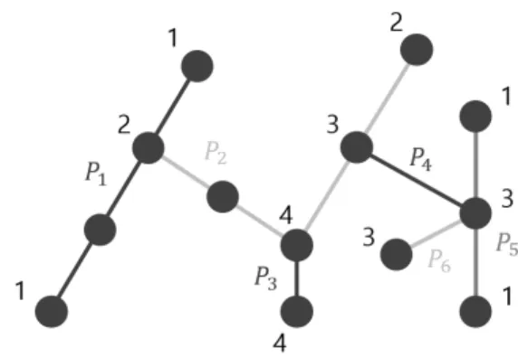
Contribution In Chapter 4 we extend the result of Batagelj et al.’s [4] in two ways;

precisely, we propose two graph classes for which the same characterization of Hamil- tonicity as Batagelj’s,p≥∆, holds. The two classes are covering graphs of trees having a self-loop at each vertex, and defined by some conditions on the labels. The condition of the first class is that the edges of Γ except self-loops can be partitioned into k paths, and for each path, the two end vertices of the path have the same label. The condition of the second class is that the edges of Γ except self-loops can be partitioned into k paths, and in each path, there are two adjacent vertices having the same label. Moreover, for both conditions we require every label to be coprime to the order of the group. For each class, one can check that it contains the class of the Cartesian product of a tree and a cycle by taking the all-one label on the self-loop at every vertex. At last, by putting these two conditions together, we obtain a larger class for which the Hamiltonicity is characterized by p≥∆.

Recall that it seems to be intractable to characterize the Hamiltonicity of the covering graphs of the small paths. Our result, however, implies that the Hamiltonicity of arbi- trarily long paths is characterized by one quite simple inequality under some conditions on the input graph, as long as the label on each self-loop is coprime to the order of the cyclic group. This is a remarkable aspect of our result.

The two conditions mentioned above, are non-trivial to check. We also propose a linear time algorithm to check if the input voltage graph satisfies each condition.

(17)

1.3 Relaxation of Constraints: Spanning Tree Problem

A spanning tree of a graphGis a spanning connected subgraph ofGhaving no cycles.

The concept of spanning tree is quite fundamental and it appears in many research areas.

Moreover, it has plenty of applications for areas such as network designs, distributed algorithms, and data structures. While it is easy to find a spanning tree (of minimum weight) in a graph, there are considerable number of hard variants. For example, finding a spanning tree having minimum or maximum number of leaves, bounded degrees, bounded diameter, and bounded number of hops, are all known to be NP-hard [23, 25]. Notice that a Hamiltonian path is equivalent to a spanning tree with minimum number of leaves.

There is a previous study concerning a spanning tree with a parity condition. Lov`asz proposed the problem, given a connected graph and a list of disjoint pairs of edges, to find a spanning tree of minimum weight such that for each two edges e, f paired in the list, both e and f are used in the tree or neither of them are used. Lov`asz showed the problem is solved in polynomial time using the linear matroid parity [45, 49].

In this thesis, we consider a variant of the problem to find a spanning tree with bounded diameter relaxing the constraint using parity. An odd depth tree is a spanning tree such that every leaf has an odd distance from a prescribed root vertex. The odd depth tree problem is to find such a tree in a given undirected graph and a root vertex². Related Topics When some parity (or a finite group) condition is added to a graph problem, it is often generalized to the problems ingroup-labeled graphs. A group-labeled graph is a pair (G, ϕ) where G is a graph and ϕ is a map from E(G) to an element of a group³. Consider a group-labeled graph associated with the group Z2 and every edge has label 1. Consider a path on the group-labeled graph in which the sum of the labels of the edges is not equal to zero. Then it corresponds to a path of odd length in the normal graph. The studies on non-zero paths or cycles in group-labeled graphs have been grown these days; packing non-zeroA-paths [14] and its reduction to matroids [54], packing non-zero cycles [38], finding a shortest non-zero A-path [39], etc.

One can suppose that an odd depth tree can be also regarded as a “non-zero” spanning tree in a group-labeled graph. However, paths and spanning trees have a crucial diﬀerence; a path is regarded as a walk on a graph, while a spanning tree is not. In other words, the operation of “taking sum of labels along a spanning tree” will make no sense. Thus it does not seem that there is a way to relate the odd depth tree problem with those studies on non-zero paths.

2One can also consider the even depth tree problem, that is, the problem to find a spanning tree such that every leaf has an even depth, which is essentially equivalent to the odd depth tree problem.

3The group-labeled graph is essentially same concept as the voltage graph. There is no mathematical diﬀerence between them, they come from diﬀerent origins.

(18)

Contribution Our results on the odd depth tree problem are as follows. For bipartite graphs, we show a Hall-type characterization of graphs having an odd depth tree. We propose a polynomial time algorithm to find an odd depth tree based on the characterization. For non-bipartite graphs, we show the problem is NP-complete. We also study the problem in directed graphs, for which we obtained similar results to the undirected case.

1.4 Organization

This thesis is organized as follows. In Chapter 2 we study the PHC problem in undirected graphs. In Chapter 3 we study the PHC problem in directed graphs. In Chapter 4 we study the HC problem in covering graphs. In Chapter 5 we study the odd depth tree problem. In Chapter 6 we summarize the results and mention future works.

(19)

(20)

Chapter 2 The PHC Problem in Undirected Graphs

In this chapter we investigate the parity Hamiltonian cycle (PHC) problem in undirected graphs. First we introduce some terminologies and notations, then formally define the PHC problem.

2.1 Preliminaries

An undirected simple graph (simply we say “graph”) G= (V, E) is given by a vertex set V (or we use V(G)) and an edge set E ⊆ (_V

2

) (or E(G)). Let δ_G(v) denote the set of incident edges to v, and let d_G(v) denote the degree of a vertex v in G, i.e., d_G(v) =|δ_G(v)|. We simply use δ(v) and d(v) without a confusion.

A walk is an alternating sequence of vertices and edges v₀e₁v₁· · ·v_ℓ₋₁e_ℓv_ℓ with an appropriate ℓ ∈ Z_≥0, such that e_i = {v_i₋₁, v_i} ∈ E for each i (1 ≤ i ≤ ℓ). Note that each vertex or edge may appear more than once in a walk. A walk is closedifvℓ =v0. A graph Gis connected if there exists a walk from uto v for any pair of verticesu, v ∈V. For a closed walk w = v₀e₁· · ·e_ℓv_ℓ, the visit number of v ∈ V, denoted by visit(v), is the number of times that v appears in the walk but counting out the last v_ℓ (since v_ℓ =v₀), i.e., visit(v) = |{i∈ {0,1, . . . , ℓ−1} |v_i =v}|.

2.1.1 Parity Hamiltonian cycle

A parity Hamiltonian cycle (PHC for short) of a graph G is a closed walk in which visit(v)≡1 (mod 2) holds for eachv ∈V. Remark again that an edge may appear more than once in a PHC w. Clearly, a graph must be connected to have a PHC, and this paper is basically concerned with connected graphs.

An edge count vector x ∈ Z^E_≥0 of a closed walk w is an integer vector where x_e for

(21)

e∈E counts the number of occurrence of e inw. Remark that visit(v) = 1

2

∑

e∈δ(v)

x_e (2.1)

holds for any closed walk. Thus, we see that a PHC is a closed walk whose edge count vector x∈Z^E_≥0 satisfies the parity condition

∑

e∈δ(v)

x_e≡2 (mod 4) (2.2)

for each v ∈V.

2.1.2 A PHC as an Eulerian cycle of a multigraph

As given an arbitrary integer vectorx∈Z^E_≥0, the parity condition (2.2) is a necessary condition for that x is an edge count vector of a PHC. In fact, the following easy but important observation provides an if-and-only-if condition.

Proposition 2.1. Let G = (V, E) be an undirected simple graph and let x ∈ Z^E_≥0 be an arbitrary integer vector. Let F = {e ∈ E | x_e > 0}, and then x is an edge count vector of a PHC in G if and only if x satisfies (2.2) and the subgraph H = (V, F) of G is connected.

As a preliminary of the proof of Proposition 2.1, we introduce an Eulerian cycle of a multigraph. For a simple graph G = (V, E) and any nonnegative integer vector x∈Z^E_≥0, let Ex be amultiset such thate ∈E appears x_e times inEx. Then, let (G,x) represent amultigraphwith a vertex setV and a multiedge setEx. Note that (G,1) = G where 1∈Z^E_≥₀ denotes the all one vector. We say (G,x) is connected if a simple graph H = (V, F) is connected where F = {e ∈ E | x_e > 0}. An Eulerian cycle of (G,x) is a closed walk which uses each element of the multiset Ex exactly once. It is celebrated fact due to Euler [19] that (G,x) has an Eulerian cycle if and only if (G,x) is connected and x satisfies the Eulerian condition

∑

e∈δ(v)

x_e≡0 (mod 2) (2.3)

holds for any v ∈V.

Proof of Proposition 2.1. The ‘only if’ part is easy from the definition. We prove the

‘if’ part. Note that x satisfies (2.3) since xsatisfies (2.2). Since H is connected by the hypothesis, the multigraph (G,x) has an Eulerian cycle w. Considering (2.1), it is not hard to see that w is a PHC since xsatisfies (2.2).

(22)

For convenience, we say x∈ Z^E_≥0 admits a PHC in G if x is an edge count vector of a PHC in G. In summary, Proposition 2.1 implies the following.

Corollary 2.2. Let G = (V, E) be an undirected simple graph and let x ∈ Z^E_≥0 be an arbitrary integer vector. Then, x admits a PHC in G if and only if (G,x) is connected and x satisfies (2.2).

2.1.3 A PHC with an edge constraint

As we repeatedly remarked, a PHC may use an edge more than once. For convenience, let PHC_z for z ∈Z>0 denote a PHC using each edge at mostz times.

2.2 Other graph terminology

This section introduces some other graph terminology which we will use in this chapter. (They will be used in the late chapters as well.)

2.2.1 Fundamental notations

A simple path is a walk w = v₀e₁v₁e₂· · ·e_ℓv_ℓ which visits every vertex (and hence every edge) at most once, whereℓ (ℓ≥0) is thelength of the path w. Similarly, asimple cycle is a closed walkw=v₀e₁v₁e₂· · ·e_ℓv₀ which visits every vertex at most once, where ℓ (ℓ≥3) is the length of the cyclew. Anodd cycle is a simple cycle of odd length.

LetG= (V, E) be a graph. For anedgesubsetF ⊆E, letG−F denote a graphH = (V, E\F). For a vertex subset S⊆V, let G−S denote the subgraph induced byV \S, i.e., G−S is given by deleting from Gall vertices of S and all edges incident to S. For convenience, we simply useG−efore∈E instead ofG−{e}, andG−v forv ∈V as well.

An edge e∈ E is abridge if its deletion increases the number of connected components of G. For a pair of graphsG and H, let G+H = (V(G)∪V(H), E(G)∪E(H)).

2.2.2 T-join

Let G = (V, E) be a graph and let T be a subset of V such that |T| is even. Then, J ⊆E is a T-join if the graph H = (V, J) satisfies

d_H(v)≡

{ 1 (mod 2) if v ∈T,

0 (mod 2) otherwise, (2.4)

for any v ∈V [52]. Notice that a graph H^′ = (T, J) may not be connected, in general.

A T-join is a generalized notion of a matching, in the sense that J is a matching when all edges in J are disjoint.

(23)

Theorem 2.3 (cf. [41]). For any graph G = (V, E) and for any T ⊆ V satisfying that

|V(C)∩T| is even for every connected component C of G, G contains a T-join.

A T-join is found in O(|V|+|E|) time (see Appendix A of [47]).

2.2.3 Edge connectivity

A graph is k-edge-connected for a positive integer k if the graph remains connected after removing arbitrary at most k−1 edges. A k-edge-connected component H of G is a maximal induced subgraph of G such thatH is k-edge-connected.

Theear decomposition is a cerebrated characterization of two-edge-connected graphs.

An ear P = v₀e₁v₁e₂· · ·e_ℓv_ℓ of a graph G is a simple path, or a simple cycle (where v₀ =v_ℓ), of length at least one where d(v_i) = 2 for each i = 1, . . . , ℓ−1 and v₀ and v_ℓ are in the same two-edge-connected component of G− {v₁, . . . , v_ℓ₋₁}, or G−e₁ when ℓ = 1. A cycle graph, which consists of a simple cycle only, is two-edge-connected. It is not diﬃcult to see that any two-edge-connected graph, except for a cycle graph, has an ear. By the definition, a graph obtained by deleting an ear P except for v₀ and v_ℓ from a two-edge-connected graph G is again two-edge-connected unless G is a cycle graph. By recursively deleting ears from a two-edge-connected graph G, we eventually obtain a single vertex. The sequence of ears obtained by the operation is called an ear decomposition of G. The following fact is well-known.

Theorem 2.4 (cf. [52]). A graph G is two-edge-connected if and only if G has an ear decomposition.

2.2.4 Graph classes

LetP_n (n≥2) denote a graph consisting of a simple path onn vertices. Notice that the length of the path P_n is n−1. Let C_n (n ≥ 3) denote a cycle graph on n vertices.

A graph is P_k-free (resp. C_k-free) if it does not contain P_k (resp. C_k) as an induced subgraph. A graph is C_≥_k-free¹ if G isC_k′-free for all k^′ ≥k. Clearly, any P_k-free graph is also P_k+1-free, as well as any C_≥_k-free graph is also C_≥_k+1-free. We can also observe that any P_k-free graph is C_≥k+1-free. However, any C_≥k-free is not included in P_l-free for any l, since a tree, which is clearlyC_≥₃-free, admits a path of any length.

Many important graph classes are known to be characterized as Pk-free or C_≥k-free.

For instance, the class of cographs is equivalent to P₄-free, chordal is equivalent to C_≥₄- free, and chordal bipartite isC_≥₆-free bipartite (cf. [10])².

1C_≥_k-free is often denoted byC_n+k-free [10].

2Here, we omit the definitions of cograph, chordal and chordal bipartite. This paper requires the properties ofP_k-free orC_≥_k-free, only.

(24)

2.3 The PHC

4

problem

It may not be trivial if the PHC problem is in NP, since the length of a closed walk is unbounded. In this section we begin with the PHC₄ problem, and give a complete characterization of the graphs which have PHC₄’s. Then we see that the PHC problem is in P as a corollary. The following is the key theorem to characterize the PHC₄ problem.

Theorem 2.5. A connected graph G= (V, E) contains a PHC if and only if the order

|V| is even or G is non-bipartite.

In fact, we prove a slightly stronger theorem (Theorem 2.6). Given a graph G = (V, E) andS ⊆V, an S-odd walk is a closed walk ofG which visits every vertex of S an odd number of times and visits every other vertex an even number of times. Clearly, a V-odd walk is a PHC of G.

Theorem 2.6. For any connected graph G and any S ⊆ V(G), G contains an S-odd walk if and only if |S| is even or G is non-bipartite. Furthermore, we can find an S-odd walk of G which uses each edge at most four times.

Proof. First, we show the ‘only if’ part. Suppose thatG= (U, V;E) is a bipartite graph, and that|S|is odd. Assume for a contradiction that Ghas anS-odd walk. Without loss of generality, we may assume that |U ∩S| is odd, and hence |V ∩S| is even since |S| is odd. Then, ∑

v∈U∩Svisit(v) is odd since visit(v) of anS-odd walk is odd for each v ∈S and |U ∩S| is odd, while ∑

v∈V∩Svisit(v) is even since |V ∩S| is even. Furthermore,

∑

v∈U\Svisit(v) is even (as well as ∑

v∈V\Svisit(v)) since visit(v) of an S-odd walk is even for each v ̸∈ S. Thus, ∑

v∈Uvisit(v) is odd while ∑

v∈V visit(v) is even. On the other hand, any closed walk ofG satisfies that∑

u∈Uvisit(u) =∑

v∈V visit(v) sinceG is bipartite. Contradiction.

Next, we show the ‘if’ part. When |S| is even, let J be an S-join ofG. Let x∈ Z^E_≥0

be given by

x_e=

{ 2 if e ∈J, 4 otherwise.

Then, (G,x) has an Eulerian cycle, which in fact an S-odd walk since J is an S-join of G.

When |S| is odd and Gis non-bipartite, let C be an odd cycle of G. Let T = (S\V(C))∪(V(C)\S),

i.e., T is the symmetric diﬀerence between S and V(C). Then, it is not diﬃcult to observe that |T| ≡ |S|+|V(C)| (mod 2) holds, and hence|T|is even since both |S|and

|V(C)|are respectively odd by the assumption. Let J^′ be aT-join ofG, and letx^′ ∈Z^E_≥0

(25)

(a) (b) (c)

Figure: 2.1: Example for the proof of Theorem 2.5 when|S|is odd andGis non-bipartite.

(a) Given graph G, vertex set S, and an odd cycle C, (b) x^′ given by (2.5) and T, (c) x^′′ given by (2.6).

be given by

x^′_e=

{ 2 if e ∈J^′,

4 otherwise, (2.5)

and then (G,x^′) satisfies the Eulerian condition, and any Eulerian cycle is aT-odd walk since J^′ is a T-join. Now, let x^′′ be given by

x^′′_e =

{ x^′_e−1 if e ∈E(C),

x^′_e otherwise. (2.6)

We remark that x_e ≤ 4 for any e ∈ E, as well as x_e > 0, where the latter observation implies (G,x^′′) is connected. Now, it is not diﬃcult to observe that (G,x^′′) has anS-odd walk since S is a symmetric diﬀerence between T and V(C).

Since a T-join of a graph is found in linear time, the following is derived from the proof of Theorem 2.6.

Corollary 2.7. A P HC₄ is found in linear time for any connected graph G if the order

|V| is even or G is non-bipartite.

Finally, we remark that Theorem 2.6 is a generalization of the following theorem due to Brigham et al. [11]. They proved it by presenting an algorithm based on a depth-first- search, without using the notion of T-join.

Theorem 2.8 (cf. [11]). Every connected graph has a closed walk visiting all vertices such that the walk visits at least |V| −1 vertices an odd number of times and uses each edge at most four times. Such a walk is found in linear time.

(26)

2.4 The PHC

z

problems when z = 1, 2, 3

In Section 2.3, we obtained a good characterization for the PHC₄ problem. This section shows that the PHC_z problem is NP-complete for each z ∈ {1,2,3}. We remark that these hardness results are independent, e.g., the fact that PHC₃ is NP-complete does not imply the fact that PHC₂ is NP-complete, and vice versa.

Theorem 2.9. The PHC1 problems is NP-complete, even when a given graph is three- connected, planar and cubic.

Proof. It is not diﬃcult to observe that the PHC₁ problem is exactly the same as the HC problem for a cubic graph. It is known that the HC problem is NP-complete even when a given graph is three-connected, planar and cubic [24].

Theorem 2.10. ThePHC₂ andPHC₃ problems are respectivelyNP-complete, even when a given graph is two-edge-connected.

Proof. It is easy to see that both problems are in NP. We reduce the HC problem for cubic graphs to the PHC problems. Let G be a two-edge-connected cubic graph, which is an input of the HC problem. Then, we construct a graph H as an input of the PHC problems, as follows (see also Figure 2.2):

• Subdivide every edge e={v, u} ∈E(G) into a path of length three, i.e., removee and add vertices ve, ue and edges {v, ve}, {ve, ue}, {ue, u}.

• For each vertex v ∈V(G), attach a cycle of length four, i.e., add verticesw_v1,w_v2, wv3 and edges {v, wv1}, {wv1, wv2}, {wv2, wv3}, {wv3, v}.

For convenience, letV denote the set of original vertices, i.e.,V =V(G), letVsdenote the set of vertices u_e, v_e added by the subdivision, and letV_c denote the set of verticesw_v1, w_v2,w_v3added by the cycle attachment, i.e.,V(H) =V∪V_s∪V_cwhere|V_s|= 2|E(G)|and

|Vc|= 3|V(G)|. Similarly, letEsdenote the set of edges{v, ve},{ve, ue},{ue, u}given by the subdivision for each v ∈V, and let E_c denote the set of edges {v, w_v1}, {w_v1, w_v2}, {w_v2, w_v3}, {w_v3, v} given by the cycle attachment for eachv ∈V, i.e.,E(H) = E_s∪E_c where |Es|= 3|E(G)| and |Ec|= 4|V(G)|.

In the following, we will prove (i) if G has an HC then H has a PHC₂, and (ii) if H has a PHC₃ then G has an HC. Since a PHC₂ is also a PHC₃, (i) implies that (i’) if G has an HC then H has a PHC₃, as well as (ii) implies that (ii’) if H has a PHC₂ then G has an HC. Thus, (i) and (ii’) imply the NP-hardness of the PHC₂ problem, and (i’) and (ii) imply the NP-hardness of the PHC₃ problem.

First, we show (i) if Ghas an HC then H has a PHC2, by presenting an edge count vector x ∈ Z^E(H)_≥0 . For the edges in E_s, set x_{_v,v_e_} = x_{_v_e_,u_e_} = x_{_u_e_,u_} = 1 if the HC uses e = {v, u} ∈ E(G), otherwise set x_{_v,v_e_} = x_{_u_e_,u_} = 2 and x_{_v_e_,u_e_} = 0. For each

(27)

edge e^′ ∈E_c, set x_e′ = 1 (see Figure 2.2, right). It is not diﬃcult to observe that (G,x) is connected and satisfies the Eulearian condition. Furthermore, an Eulerian cycle of (G,x) visits every vertex of V(H) an odd number of times; it visits every vertex of V exactly three times, and every other vertices exactly once. Thus, x admits a PHC₂ of H.

Next, we show (ii) if H has a PHC₃ then G has an HC. Let x be the edge count vector of the PHC3 of H. In order to visit each vertex of Vc an odd number of times, we can observe that (x_{_v,w_v1_}, x_{_w_v1_,w_v2_}, x_{_w_v2_,w_v3_}, x_{_w_v3_,v_}) should be (1,1,1,1) or (3,3,3,3) for each cycle attached to v ∈V since d_H(v^′) = 2 for v^′ ∈V_c. Similarly, there are three possible assignments of (x_{_v,v_e_}, x_{_v_e_,u_e_}, x_{_u_e_,u_}) for the subdivided path betweenv andu (i.e., {v, u} ∈ E(G)), namely (1,1,1), (2,0,2) or (3,3,3). Recall the hypothesis that G is cubic, and let a, b, c ∈E(G) denote the edges incident to v in G, meaning that three subdivided paths are incident to v ∈ V in H. To be precise, dH(v) is 5, where {v, va}, {v, v_b},{v, v_c}inE_s and{v, w_v1},{v, w_v3}inE_c are incident tov. The assumption that xis the edge count vector of a PHC₃, which visits every vertex an odd number of times, implies that

x_{_v,v_a_} +x_{_v,v_b_}+x_{_v,v_c_}+x_{_v,w_v1_}+x_{_v,w_v3_} ≡2 (mod 4) holds. As we saw, x_{_v,w_v1_} =x_{_v,w_v3_} = 1 or 3 hold, which implies

x_{_v,v_a_}+x_{_v,v_b_}+x_{_v,v_c_} ≡0 (mod 4).

Then, the possible multisets of values of {{x_{_v,v_a_}, x_{_v,v_b_}, x_{_v,v_c_}}} are {{1,1,2}} or {{3,3,2}} where {{·}} denotes a multiset. This means that exactly two of subdivided paths incident to each vertex of V are assigned (1,1,1) or (3,3,3), while the other is assigned (2,0,2). Now it is easy to observe that we obtain an HC ofGby choosing edges corresponding to (1,1,1) or (3,3,3) paths.

2.4.1 The PHC₃ problem for four-edge-connected graphs

The PHC₃ problem is NP-complete for two-edge-connected graphs, as we have shown in Theorem 2.10. For four-edge-connected graphs, we obtain the following.

Theorem 2.11. A four-edge-connected graph G= (V, E) contains a PHC₃ if and only if the order |V| is even or G is non-bipartite.

To prove Theorem 2.11, we use the following celebrated theorem.

Theorem 2.12 ([46, 28]). Every four-edge-connected graph has two edge disjoint span- ning trees.

(28)

Figure: 2.2: A PHC₂ around vertexv.

Proof of Theorem 2.11. The ‘only-if’ part follows from that of Theorem 2.5. We show the ‘if’ part, in a constructive way. Suppose that G is four-edge-connected. Then, let τ and τ^′ be a pair of edge disjoint spanning trees of G, implied by Theorem 2.12.

Intuitively, we construct a closed walk onτ, and control the parity condition using edges inτ^′, then we obtain a PHC₃.

Let x∈Z^E_≥0 be given by

xe =

{ 2 if e∈E(τ),

0 otherwise. (2.7)

Then, (G,x) is connected, and has an Eulerian cycle, sayw. LetS be the set of vertices with even degree in τ, i.e., S is the entire set of vertices each of which w visits an even number of times. We also remark that |V \S| is even, by the handshaking lemma. In the following, we consider two cases whether |V| is even or odd.

If |V| is even, then |S| is even. Let J ⊆E(τ^′) be anS-join in the tree τ^′. Then, let x^′ ∈Z^E_≥₀ be defined by

x^′_e=

{ x_e+ 2 if e∈J,

x_e otherwise. (2.8)

It is easy to see thatx^′ satisfies the parity condition (2.2) for each vertex of V since J is an S-join. Clearly (G,x^′) is connected, and x^′ admits a PHC by Corollary 2.2. Notice that J ⊆E(τ^′) is disjoint withE(τ), meaning that (2.7) and (2.8) imply that x^′_e≤2 for eache ∈E. We obtain the claim in the case.

If |V| is odd, then |S| is odd. By the hypothesis, G is non-bipartite and hence G

(29)

contains an odd cycle, sayC. Let

T = (S\V(C))∪(V(C)\S),

i.e., T is the symmetric diﬀerence between S and V(C). Then, it is not diﬃcult to observe that |T| ≡ |S|+|C| (mod 2) holds, and hence |T| is even since both |S| and

|C| are respectively odd by the assumption. Let J^′ ⊆ E(τ^′) be an T-join of τ^′, and let x^′′∈Z^E_≥0 be defined by

x^′′_e =

{ x_e+ 2 if e∈J^′,

xe otherwise. (2.9)

It is not diﬃcult to see that (G,x^′′) has a (V \V(C))-odd walk. Finally, we modify x^′′

tox^′′′ ∈Z^E_≥0 by

x^′′′_e =

{ x^′′_e+ 1 if e∈E(C),

x^′′_e otherwise, (2.10)

and then we obtain a PHC₃.

It is known (cf. [52]) that a pair of edge disjoint spanning treesτ andτ^′ in a four-edge- connected graph is found in polynomial time (e.g., O(|E(G)|²) time, due to Roskind, Tarjan [51]). Thus, the proof of Theorem 2.11 also implies a polynomial time (e.g., O(|E(G)|²)) algorithm to find a PHC₃ in a four-edge-connected graphG.

2.5 The PHC

₃

Problem for Two-Edge-Connected Graphs

The PHC₃ problem is NP-complete for two-edge-connected graphs (Theorem 2.10), while it is solved in polynomial time for anyfour-edge-connected graph (Theorem 2.11).

We devote this section to dig into the PHC₃ problem in two-edge-connected graphs (which includes the class of three-edge-connected graphs). The goal of this section is to establish the following theorem.

Theorem 2.13. Suppose that a two-edge-connected graphGisP₆-free orC_≥₅-free. Then, G= (V, E) contains a PHC₃ if and only if the order |V| is even or G is non-bipartite.

As mentioned before,C_≥₅-free contains some important graph classes such as chordal (equivalent toC_≥₄-free), chordal bipartite (equivalent toC_≥₅-free bipartite), and cograph (equivalent to P4-free). We also remark that the Hamiltonian cycle problem is NP- complete for C_≥₄-free graphs, as well as P₅-free graphs (cf. [10]).

2.5.1 All-roundness : Preliminary

We introduce the notion of theall-roundnessof a graph. This notion is used throughout the rest part of this section to characterize the graphs having PHC₃’s.

(30)

Generalized problem

Section 2.5 is actually concerned with the following problem, which is a slight generalization of the PHC3 problem.

Problem 1. Given a graph G = (V, E) and a map f: V → {0,1,2,3}, find x ∈ {0,1,2,3}^E satisfying the conditions that

∑

e∈δ(v)

x_e≡f(v) (mod 4) for any v ∈V, (2.11)

(G,x) is connected. (2.12)

Clearly, the PHC₃ problem is given by setting f(v) = 2 for any v ∈V (recall Corol- lary 2.2). For convenience, we call x ∈ {0,1,2,3}^E a mod-4 f-factor of G if x satisfies (2.11). A mod-4f-factorx∈ {0,1,2,3}^E isconnectedif it satisfies (2.12), i.e., Problem 1 is a problem to find a connected mod-4 f-factor. We remark the following two facts.

Proposition 2.14. A graph G = (V, E) has a mod-4 f-factor only when the map f satisfies that

∑

v∈V

f(v) is even. (2.13)

Proof. Summing up the both sides of (2.11) over V, we obtain

∑

v∈V

f(v)≡∑

v∈V

∑

e∈δ(v)

x_e (mod 4). (2.14)

It is not diﬃcult to see that ∑

v∈V

∑

e∈δ(v)

x_e= 2∑

e∈E

x_e (2.15)

holds, in an analogy with the handshaking lemma, that is∑

v∈V

∑

e∈δ(v)1 = ∑

e∈E2. By (2.14) and (2.15), we obtain that

∑

v∈V

f(v)≡2∑

e∈E

x_e (mod 4) which implies the claim.

We will later show in Lemma 2.23 that (2.13) is also suﬃcient for any connected non-bipartite graph to have a mod-4 f-factor. For bipartite graphs, we need an extra necessary condition on f.

Characterizations of Graphs for Eﬃcient Algorithms

有限群を用いた計算困難なグラフ問題の緩和と，効 率的アルゴリズムのためのグラフの特徴づけ

Characterizations of Graphs for Eﬃcient Algorithms

Hiroshi Nishiyama

Abstract

Acknowledgment

Table of Contents

Chapter 1 Introduction

1.1 Relaxation of Constraints: Parity Hamiltonian Cycle Prob- lem

1.2 Relaxation of “For Any” Condition : HC’s in Covering Graphs

1.3 Relaxation of Constraints: Spanning Tree Problem

1.4 Organization

Chapter 2

The PHC Problem in Undirected Graphs

2.1 Preliminaries

2.2 Other graph terminology

2.3 The PHC

problem

2.4 The PHC

problems when z = 1, 2, 3

2.5 The PHC

Problem for Two-Edge-Connected Graphs

有限群を用いた計算困難なグラフ問題の緩和と，効率的アルゴリズムのためのグラフの特徴づけ