nuclear effective field theory on a lattice on the basis of renormalization group analysis

九州大学学術情報リポジトリ

Kyushu University Institutional Repository

格子上の核子系有効場理論に対する繰り込み群解析 に基づいた再加重法

佐々部, 悟

https://doi.org/10.15017/1806808

出版情報：Kyushu University, 2016, 博士（理学）, 課程博士 バージョン：

権利関係：Fulltext available.

Reweighting method for

nuclear effective field theory on a lattice on the basis of renormalization group analysis

SASABE Satoru

Theoretical Nuclear Physics, Department of Physics Graduate School of Science, Kyushu University 744, Motooka, Nishi-Ku, Fukuoka 819-0395, Japan

February, 2017

Abstract

Recent development of experiments with radioactive isotope beams and observations of two-solar-mass neutron stars questioned existing knowledge of nuclear physics and have attracted extensive attention. Most ideal theoretical approach to figure out prop- erties of these exotic nuclear systems is so-called lattice quantum chromodynamics (LQCD) which is the first-principle calculation of QCD. However, LQCD has difficul- ties in describing finite nuclei and nuclear matter. For finite nuclei, high computational costs are required. For nuclear matter, the notorious fermion sign problem caused by finite chemical potential prevents the probability interpretation of the integrand of path integrals in performing Monte Carlo simulations.

Since typical energy scale of nuclear physics is smaller than that of QCD, nuclear effective field theory (NEFT), i.e., low-energy effective theory of QCD, provides an alternative approach. By defining NEFT on a lattice and performing lattice simula- tions in the same manner as in LQCD, we can study finite nuclei and nuclear matter.

However, when we try to increase the physical cutoff, the momentum scale below which effective field theory is valid, fermion sign problem occurs like LQCD with finite chemical potential.

In this dissertation, we propose a method to avoid the sign problem of NEFT on a lattice. The method is the same as the reweighting method which is often used in LQCD calculations with finite chemical potential except for how to determine the reference determinant. Unlike QCD, there is a hierarchy of importance of operators in NEFT. We perform renormalization group analysis to determine which operators are important for low-energy physics. On the basis of the analysis, we distinguish the operators which are relevant in low-energy physics and thus should be included in the reference determinant from those which may not be. To assess the method we propose, we perform lattice simulations and evaluate its effectiveness.

This dissertation is based on the following two papers:

• Numerical study of renormalization group flows of nuclear effective field theory without pions on a lattice,

K. Harada, S. Sasabe, and M. Yahiro, Phys. Rev. C 94, 024004 (2016).

• Reweighting method for nuclear effective field theory on a lattice: an application of renormalization group analysis,

S. Sasabe, K. Harada, and M. Yahiro (unpublished).

i

Acknowledgement

I would like to express thanks to Prof. Masanobu Yahiro, Prof. Koji Harada, Prof.

Atsushi Nakamura, Associate Prof. Yoshifumi R. Shimizu, Assistant Prof. Takuma Matsumoto, Prof. Hiroshi Suzuki, and everyone who has supported me in my college life.

This work was supported by the Research Fellowship of the Japan Society for the Promotion of Science (JSPS) for Young Scientists (Grant No. 26 · 5861).

iii

Contents

Abstract i

Acknowledgement iii

1 Introduction 1

1.1 Current status of nuclear physics . . . . 1

1.2 NEFT on a lattice . . . . 2

1.3 Overview . . . . 4

2 Renormalization group analysis 5 2.1 NLO NEFT without pions in the continuum . . . . 5

2.2 RG flows with the lattice-regularized integrals . . . . 8

2.3 Ground-state wave function and the ANC . . . . 12

2.4 NLO NEFT without pions on a lattice . . . . 15

3 Reweighting Method 27 3.1 Fermion sign problem . . . . 27

3.2 Fermion matrix on a lattice . . . . 30

3.3 Reweighting method based on RG analysis . . . . 33

3.4 Computational strategy . . . . 36

3.5 Numerical results . . . . 37

4 Summary 53

v

List of Figures

2.1 The flow and the fixed points of the NLO NEFT in the X-Y plane obtained by using a sharp momentum cutoff in the continuum formulation 9 2.2 The flow and the fixed points of the NLO NEFT in the X-Y plane

obtained by using a lattice regularization with the three-point formula . 10 2.3 The flow and the fixed points of the NLO NEFT in the X-Y plane

obtained by using a lattice regularization with the five-point formula . 11 2.4 The cutoff dependence of the binding energy and the ANC . . . . 14 2.5 The rotational symmetry breaking in the asymptotic behavior of the

wave function . . . . 19 2.6 The flow of the NLO NEFT in the strong coupling phase in the X-Y

plane obtained by numerical diagonalization of the Hamiltonian defined on a lattice with the five-point formula . . . . 20 2.7 The difference of the calculated ground-state energies with N

= 14 and

N

= 16 and that with N

= 16 and N

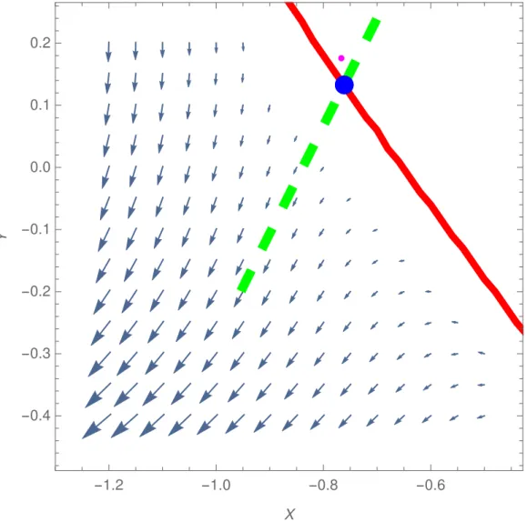
= 18 as functions of X and Y . 21 2.8 The flow calculated with the five-point formula with the ridge line, the

nontrivial fixed point, and the relevant direction . . . . 22 2.9 The flow calculated with the three-point formula with the ridge line,

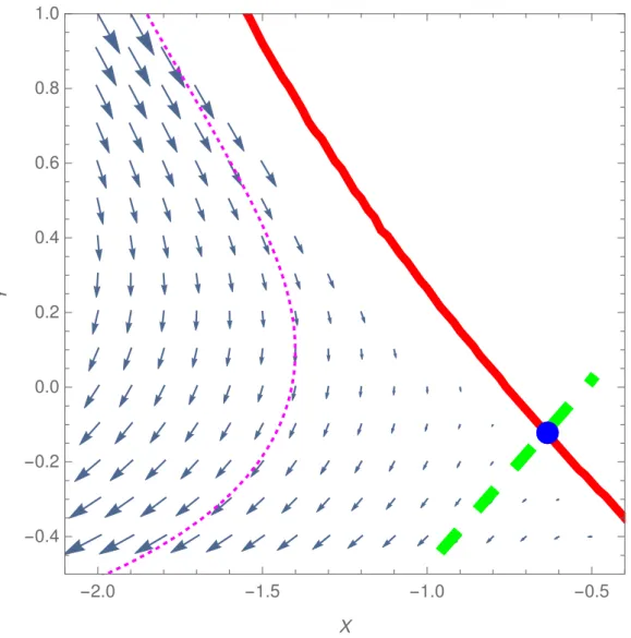
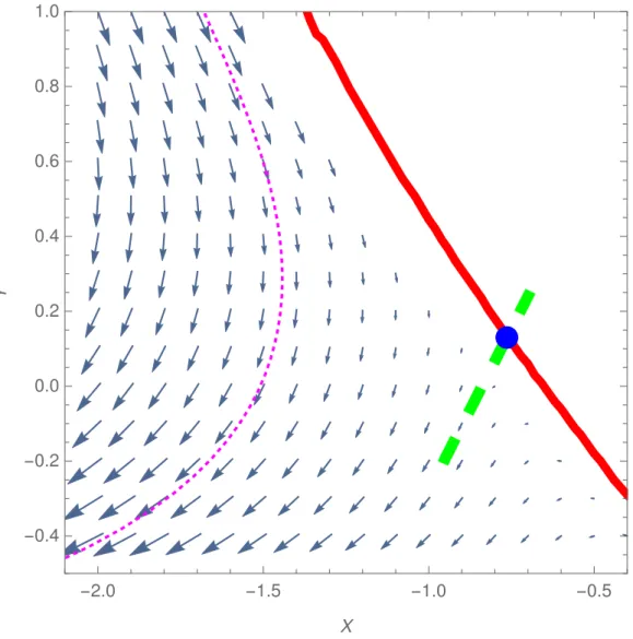
the nontrivial fixed point, and the relevant direction . . . . 23 2.10 The flow line corresponding to deuteron calculated with the five-point

formula . . . . 24 2.11 The flow line corresponding to deuteron calculated with the three-point

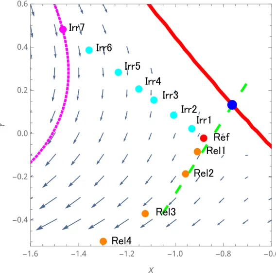
formula . . . . 25 3.1 The Physical point corresponding to deuteron and the reference point

of the reweighting method . . . . 35 3.2 The reweighting factor for the point labeled as “Irr7” . . . . 39 3.3 The reweighting factor for the point labeled as “Irr7” on the complex

plane after tuning the chemical potential µ . . . . 40 3.4 The standard deviation of the absolute value of the reweighting factor

for the point labeled as “Irr7” . . . . 40 3.5 The standard deviation of the absolute value of the reweighting factor

for the point labeled as “Irr1” . . . . 41 3.6 The standard deviation of the absolute value of the reweighting factor

for the point labeled as “Irr2” . . . . 42 3.7 The standard deviation of the absolute value of the reweighting factor

for the point labeled as “Irr3” . . . . 42 3.8 The standard deviation of the absolute value of the reweighting factor

for the point labeled as “Irr4” . . . . 43

vii

viii LIST OF FIGURES 3.9 The standard deviation of the absolute value of the reweighting factor

for the point labeled as “Irr5” . . . . 43 3.10 The standard deviation of the absolute value of the reweighting factor

for the point labeled as “Irr6” . . . . 44 3.11 The standard deviation of the absolute value of the reweighting factor

for the point labeled as “Rel1” . . . . 44 3.12 The standard deviation of the absolute value of the reweighting factor

for the point labeled as “Rel2” . . . . 45 3.13 The standard deviation of the absolute value of the reweighting factor

for the point labeled as “Rel3” . . . . 45 3.14 The standard deviation of the absolute value of the reweighting factor

for the point labeled as “Rel4” . . . . 46 3.15 The direction dependence of the standard deviation for ν ≃ − 40 MeV . 47 3.16 The direction dependence of the standard deviation for ν ≃ − 36 MeV . 48 3.17 The direction dependence of the standard deviation for ν ≃ − 32 MeV . 48 3.18 The direction dependence of the standard deviation for ν ≃ − 28 MeV . 49 3.19 The direction dependence of the standard deviation for ν ≃ − 24 MeV . 49 3.20 The direction dependence of the standard deviation for ν ≃ − 20 MeV . 50 3.21 The direction dependence of the standard deviation for ν ≃ − 16 MeV . 50 3.22 The standard deviations of the absolute value of the reweighting factor

for the point labeled as “Irr7” obtained with renormalization group

analysis and naive dimensional analysis . . . . 51

List of Tables

2.1 Locations of the nontrivial fixed point . . . . 12 2.2 Constants for the RW equations . . . . 12 3.1 Labels for various sets of a

and r

. . . . 34

ix

Chapter 1 Introduction

First, we review the current status of nuclear physics in Sec. 1.1. In Sec. 1.2, we introduce nuclear effective field theory (NEFT) and explain its application on a lattice.

Finally, we show overview of this dissertation.

1.1 Current status of nuclear physics

Recently, main subject of nuclear physics research is switched over from stable nuclei to exotic nuclei with marked improvement in experimental equipment. A prominent example of exotic nuclei is halo nuclei which are unstable nuclei and locate in the vicinity of the drip line in the nuclear chart. Due to the fact that a few nucleons of halo nuclei spread out widely, halo nuclei have larger radii compared with stable nuclei with the same mass contrary to the relation r ≃ 1.2A

between radius r and mass number A which reflects the saturation property. Typical example of halo nuclei is

11

Li whose radius is as large as that of

Pb in spite of the fact that

Li has much smaller mass number than

Pb.

Another exotic nuclear system is neutron stars. Neutron stars are compact and dense stars formed in supernova explosions and composed mainly of neutrons. The typical values of their radii and the masses are about 10 km and 1.4 solar mass, respectively. At the center of neutron stars the density is expected to be several times normal nuclear density due to the neutron degeneracy pressure against gravitational collapse. Such high density nuclear matter does not realize in the usual circumstances since nuclear matter becomes stable at the saturation density; the strong external force, i.e., gravitation, makes it realized.

Physics of these exotic nuclear systems received extensive attention as new sub- jects which enrich our understanding of nuclear physics. The most popular theoretical approaches to investigate unstable nuclei and neutron star matter are quantum many body calculations starting from effective interactions. Since effective interactions are determined by systematic analysis of properties of stable nuclei, the application of effective interactions to such extreme systems is accompanied by uncertainties. Fur- thermore, the discovery of two-solar-mass neutron stars [12, 2] requires modification of the equation of state obtained with the existing effective interactions.

One of the ideal theoretical approaches which describe nuclear systems without un- certainties is so-called lattice quantum chromodynamics (LQCD). With LQCD, one can figure out properties of a system with strong interaction by defining quantum chro- modynamics on a lattice and performing Monte Carlo simulation. Although LQCD

1

2 CHAPTER 1. INTRODUCTION is a powerful tool for us to understand the physics of strongly interacting systems, its application to finite nuclei and nuclear matter is very difficult at present. For finite nuclei, high computational costs are required due to the following reasons. First of all, the number of quark contractions which should be taken in the correlators of nuclei increases rapidly as the number of nucleons of the nuclei increases. Some contraction algorithms [14, 13, 24] have been proposed, but solved the difficulty only partially.

Second, a lattice with large spatial volume which is capable of accommodating finite nuclei is required. Third, a lattice with extremely large distance in temporal direction is necessary to separate the signal for the ground state from that for excited states.

Recall that the typical energy difference between the ground state and excited states is O (1) MeV for finite nuclei, whereas that for hadrons is O (100) MeV. For these reasons, LQCD simulations for finite nuclei is prohibitively expensive. For nuclear matter, the notorious fermion sign problem caused by finite chemical potential makes the proba- bility interpretation of the integrand of path integrals impossible. To overcome these difficulties, a great deal of effort has been made for many years.

We therefore take an alternative approach to describe finite nuclei and nuclear matter; nuclear effective field theory on a lattice, which I will describe in the next section.

1.2 NEFT on a lattice

Since the seminal work on the low-energy effective field theory of nucleons, nuclear effective field theory (NEFT), by Weinberg [49, 50, 51], extensive investigation has been performed; see Refs. [15, 43] for the reviews. In contract to QCD in which the fundamental degrees of freedom are quarks and gluons, NEFT describes systems with strong interaction at low-energies in terms of low-lying hadrons, such as nucleons and pions. In NEFT, there is a certain momentum scale, the physical cutoff Λ

below which NEFT is expected to be equivalent to QCD. The effects of heavier hadrons than Λ

, the processes with momenta higher than Λ

, and the internal structure of the hadrons are integrated out, represented by an infinite number of local operators which satisfy the same symmetries as QCD holds, and have been encoded in the coupling constants of the interactions, low-energy constants. For example, the effects of heavy-meson exchange processes between two nucleons are represented by local four-nucleon operator without derivatives and those with even number of derivatives.

It is noteworthy that even if pions are included in NEFT, the exchange of the pion with momentum transfer higher than the cutoff is represented as local four-nucleon (and 2n-nucleon, in general) operators.

There is a hierarchy of importance among an infinite number of local operators in NEFT. Classically, the contribution of an operator with a canonical dimension d is of (Q/Λ

)

order, where Q represents the typical momentum scale of interest.

Thus, operators are classified through naive dimensional analysis into the leading

order, the next-to-leading order, and so on. Based on the hierarchy of operators,

the accuracy of NEFT can be improved systematically by introducing higher order

operators. In most cases, the ordering of importance given by naive dimensional

analysis is valid. However, quantum fluctuations change the situation drastically in

some cases. In such cases, a “quantum” version of dimensional analysis is required,

and it is renormalization group analysis that provides it. Renormalization group

1.2. NEFT ON A LATTICE 3 analysis in which how the low-energy constants vary as a function of the cutoff is investigated reveals that the contribution of an operator with a canonical dimension d changes from of (Q/Λ

)

order to of (Q/Λ

)

order where ν is called scaling dimension. An operator with positive ν is called relevant, whereas that with negative ν is called irrelevant. Of course, as the typical momentum scale of interest decreases, relevant operators play important role and the effect of irrelevant operators becomes insignificant.

Although the early investigations exclusively employed continuous, semi-analytic approach based on the Lippmann-Schwinger (LS) equation, the Faddeev equation, etc., the methods of numerical simulation on a lattice have been developed recently [38, 4, 5, 1, 17, 34, 16, 42, 35, 52, 23, 22, 48, 33]; see Ref. [37] for the review. On a lattice, the cutoff in momentum is given by the lattice constant a as π/a. Thus, unlike LQCD, the continuum limit in lattice NEFT should not be taken so that the cutoff does not exceed the physical cutoff.

Lattice simulation of NEFT has several advantages. First of all, in the framework of NEFT on a lattice, the investigation of many-nucleon systems can be performed without suffering from complications due to the increase of the number of nucleons.

Recall that the Faddeev equation for three nucleons is more complex than the LS equation for two nucleons, and the Faddeev-Yakubovsky equation for four nucleons is even more complex. Lattice formulation does not have this kind of complication.

However, there is a drawback; Construction of many-nucleon operators which are nec- essary when, for example, the correlators of nuclei are calculated becomes complicated corresponding to the increase of the number of nucleons. So far, considerably large nuclei to

Si have already been investigated on a lattice [18, 34, 16]. Second, arbi- trarily complicated pion interactions can be taken into account in lattice simulations, just like arbitrarily complicated interactions of gluons can be incorporated in LQCD.

Therefore, it has potential of the calculations with the nonlinearly realized exactly chi- ral symmetric interactions of pions. Note that the truncation of pion interactions at a finite order which is often employed in semi-analytic calculations inevitably breaks chiral symmetry. Third, it is straightforward to make the system contact to a heat reservoir and/or to a particle reservoir. So, it allows us to study finite temperature, finite density system. It is noteworthy that finite chemical potential does not give rise to fermion sign problem in the case that nucleons are dealt with as non-relativistic particles unlike LQCD where relativistic quarks inhabit [7].

Meanwhile, pion interactions which should be taken into account with increasing the physical cutoff Λ

cause the fermion sign problem [6]. Also, Including higher order contact interactions sometimes brings about the sign problem. This fact prevent us from increasing the cutoff. To increase the cutoff and to include higher order operators are important for NEFT to be more accurate and more applicable.

In this study, we propose a method to avoid the sign problem and assess its validity.

Although we confine ourselves to considering the next-to-leading order (NLO) NEFT

without pions in this study, in principle, the method we propose can be applied to

the case where pion interactions and/or higher order operators are included. Note

that the long-distance parts of pion interaction, corresponding to the pion exchanges

with the momenta below the cutoff Λ, are irrelevant in low-energy physics, whereas

the short-distance parts are included in the contact interactions in accordance with

the general principle of renormalization [28]. The study is an important step toward

the chirally symmetric NEFT with pions on a lattice.

4 CHAPTER 1. INTRODUCTION

1.3 Overview

In this dissertation, we develop a reweighting method based on renormalization group analysis. For this purpose, we consider the NLO NEFT without pions since it has both parameter regions where the sign problem occurs and does not.

This dissertation is organized as follows. In Chap. 2, we perform the renormal- ization group (RG) analysis of the NLO NEFT without pions defined on a lattice by diagonalizing the lattice Hamiltonian numerically. The obtained RG flows are com- pared with the flow in the continuum and the flows obtained analytically with lattice- regularized integrals. Based on the RG analysis performed in Chap. 2, we develop the reweighting method and assess its effectiveness by executing Monte Carlo simula- tions in Chap. 3. The validity of the method is confirmed by comparing the resulting reweighting factor in the irrelevant direction with that in the relevant direction for various values of chemical potential. In addition to this, we compare the reweighting method based on the RG analysis with that based on the naive dimensional analysis.

Finally, Chap. 4 is devoted to a summary.

Chapter 2

Renormalization group analysis

2.1 NLO NEFT without pions in the continuum

We start with the following isospin SU(2) symmetric Lagrangian of the NLO NEFT without pions:

L = N

(

i∂

+ ∇

2M

)

N − C

(

N

P

N )

(

N

P

N ) +C

[(

N

P

N )

(

N

P

← → ∇

N )

+ H.c.

]

, (2.1)

where N represents the nucleon field, M is the nucleon mass, and ← →

∇

= ← −

∇ · ← −

∇ − 2 ← −

− ∇ ·

→ ∇ + − → ∇ · − → ∇ corresponds to the momentum transfer squared in the center-of-mass frame of two incoming or outgoing nucleons. P

is a projection operator for a specific channel of the two-nucleon states; for the

S

(spin-triplet) channel, P

= σ

σ

τ

/ √

8 where σ

and τ

are spin and isospin Pauli matrices, respectively. The term represented by the momentum independent four-nucleon operator is the leading-order (LO) interaction, whereas the term represented by the four-nucleon operator with two spatial derivatives is the next-to-leading order (NLO) interaction. Thus, C

and C

are the low-energy constants for LO and NLO operators, respectively.

The S-wave Lippmann-Schwinger (LS) equation for the off-shell center-of-mass nucleon-nucleon (N N ) scattering amplitude derived form the Lagrangian, Eq. (2.1), is given by

− i A (p

, p

, p

) = − iV (p

, p

) +

∫ d

k

(2π)

[ − iV (k, p

)]

× iG(p

, k) [

− i A (p

, p

, k) ]

, (2.2) where V is the vertex in momentum space,

V (p

, p

) = C

+ 4C

(p

+ p

), (2.3) G(k) represents the propagator,

G(p

, k) = 1

p

− k

/M + iϵ , (2.4)

p

is the off-shell center-of-mass energy of the system, and p

and p

are half the relative momenta in the incoming and outgoing two-nucleon states, respectively.

5

6 CHAPTER 2. RENORMALIZATION GROUP ANALYSIS The LS equation can be solved formally as

A (p

, p

) = C

+ 4C

(p

+ p

) + (C

α(p

) + 4C

β(p

)) + 4C

α(p

)p

, (2.5) where we suppressed the argument p

and introduced functions α(p

) and β(p

),

α(p

) =

∫ d

k

(2π)

G(k) A (p, k), (2.6)

β(p

) =

∫ d

k

(2π)

k

G(k) A (p, k). (2.7) By multiplying Eq. (2.5) by G(p

)(2π)

and p

G(p

)(2π)

and integrating over p

, we obtain the system of linear equations for α(p

) and β(p

),

( 1 − C

I

− 4C

I

− 4C

I

− C

I

− 4C

I

1 − 4C

I

) ( α(p

) β(p

)

)

=

( C

I

+ 4C

I

+ 4C

I

p

C

I

+ 4C

I

+ 4C

I

p

)

, (2.8)

where we have introduced the integrals, I

= − M

∫ d

k (2π)

| k |

| k |

+ µ

, (2.9)

with

µ = √

− M p

− iϵ. (2.10)

The system of linear equations can be solved as α(p

) = D

[

C

I

+ 4C

(I

− 4C

I

+ 4C

I

I

) + 4C

I

p

]

, (2.11) β(p

) = D

[

C

I

+ 4C

I

+ 4C

(I

− 4C

I

+ 4C

I

I

)p

]

, (2.12) where D represents the determinant of the coefficient matrix,

D = 1 − C

I

− 8C

I

+ 16C

I

− 16C

I

I

. (2.13) By substituting Eqs. (2.11) and (2.12) into Eq. (2.5), we obtain the N N scattering amplitude [21, 45, 26] as

A (p

, p

) = x + y (

p

+ p

)

+ zp

p

, (2.14) with

x = (

C

+ 16C

I

)

/D, (2.15)

y = 4C

(1 − 4C

I

)/D, (2.16)

z = 16C

I

/D. (2.17)

Note that the integrals I

we introduced are divergent and thus we need to regularize them in some way. If we employ a sharp momentum cutoff Λ, they are expressed as

I

= − M 2π

∫

0

dk k

k

+ µ

. (2.18)

2.1. NLO NEFT WITHOUT PIONS IN THE CONTINUUM 7 The Wilsonian RG analysis of the off-shell N N scattering amplitude can be per- formed elegantly by introducing the energy-dependent redundant operators, which can be eliminated by making use of equations of motion [3, 26, 27]. However, we consider the on-shell formulation since it is simpler and sufficient for our present pur- pose. See Ref. [26] for the relation between the two formulations. At low energies, the inverse of the on-shell amplitude can be written in powers of the momentum p = √

M p

= | p

| = | p

| as A

on−shell

= − M 4π

[

− 1 a

+ 1

2 r

p

+ O (p

) − ip ]

. (2.19)

This expansion is known as the effective range expansion and the low-energy parame- ters such as the scattering length a

and the effective range r

characterize the system at low energies.

By performing the effective range expansion for the obtained scattering amplitude, we obtain the scattering length and the effective range as

M 4π

1

a

= MΛ 2π

[

θ

+ (1 + θ

Y )

X − θ

Y

]

, (2.20)

M 4π

r

2 = M

2π

Λ [

− R(0) + Y (2 + θ

Y )(1 + θ

Y )

(X − θ

Y

)

]

, (2.21)

where, according to Seki and van Kolck [46], we have introduced dimensionless cou- pling constants X and Y defined by

C

= 2π

M Λ X, 4C

= 2π

M Λ

Y, (2.22)

the constants θ

(n = 1, 3, 5) and the function R(x) defined by I

= − M λ

2π

[

θ

+ ( p

Λ

)

R ( p

Λ

)]

− iM

4π p, (2.23)

L

≡ − M

∫ d

k

(2π)

= − M Λ

2π

θ

, (2.24)

L

≡ − M

∫ d

k

(2π)

| k |

= − M Λ

2π

θ

. (2.25)

If the regularization with the sharp momentum cutoff Λ is employed, θ

= 1, θ

= 1

3 , θ

= 1

5 , R(0) = − 1. (2.26) It is noteworthy that the expressions Seki and van Kolck obtained do not contain the terms higher than linear in Y of Eqs. (2.20) and (2.21) as a result of their perturbative treatment of the NLO interaction.

We obtain the following RG equations by imposing the condition that a

and r

8 CHAPTER 2. RENORMALIZATION GROUP ANALYSIS are independent of Λ:

Λ dX

dΛ = X (1 + 6θ

Y ) + Y

(

5θ

+ 3θ

X + 3θ

θ

Y ) + X − θ

Y

(1 + θ

Y )

[ − R(0) (θ

X + θ

Y ) (

X − θ

Y

) +θ

{

θ

Y

(3 + 2θ

Y ) + X [1 + 2θ

Y (2 + θ

Y )] }]

, (2.27) Λ dY

dΛ = 3Y (

1 + θ

2 Y

)

(1 + θ

Y ) + X − θ

Y

2(1 + θ

Y )

[ − R(0)X + 4θ

Y + { R(0)θ

+ 2θ

θ

} Y

]

. (2.28)

We find the fixed points which make both the right-hand side of Eq. (2.27) and that of Eq. (2.28) zero at the same time, and locate the nontrivial fixed point which is responsible for the “unnaturally” large scattering length in the

S

channel as

(X

, Y

) = [ 3

5 (

4 − 3 √ 3

) , 3

2

( − 2 + √ 3

)]

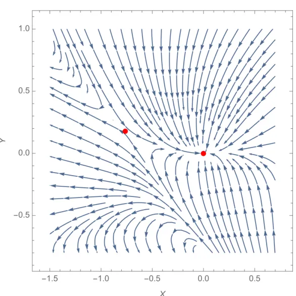
= ( − 0.717691 . . . , − 0.401924 . . .). (2.29) In Fig. 2.1, we show the obtained trivial and nontrivial fixed points together with the RG flow. The arrows indicate the directions in which X and Y evolve as the cutoff decreases.

Note that the location of the fixed point and the flow are not universal, while the existence of the nontrivial fixed point and the scaling dimensions, which are the eigenvalues of the linearized RG equations in the vicinity of the nontrivial fixed point, are universal. We see the fact that the location of the fixed point and the flow depend on the details of the regularization scheme and how they vary as the regularization is changed in the following sections.

2.2 RG flows with the lattice-regularized integrals

In this section, we consider to regularize the integrals defined by Eq. (2.9) with a lattice following Seki and van Kolck [46] to obtain RG flows which approximate those on a lattice. We suppose the lattice whose volume is infinite and lattice constant is a.

We restrict the interval of integration to be the first Brillouin zone,

− π

a ≤ k

≤ π

a (i = 1, 2, 3), (2.30)

and replace the momentum square | k |

coming from the Laplacian ∇

in the continuum with the corresponding discretized one obtained with the three-point formula,

| k |

→ 4 a

∑

i=1

sin

( k

a

2 )

. (2.31)

With this prescription, for example, the integral I

is given as I

= M

a

∏

i=1

[∫

dk

2π

] 1

p

− 4 ∑

i=1

sin

(k

/2) + iϵ , (2.32)

2.2. RG FLOWS WITH THE LATTICE-REGULARIZED INTEGRALS 9

-1.5 -1.0 -0.5 0.0 0.5

-0.5 0.0 0.5 1.0

X

Y

Figure 2.1: The flow and the trivial and nontrivial fixed points of the NLO NEFT in the X-Y plane obtained by using a sharp momentum cutoff in the continuum formulation. The arrows indicate the directions in which X and Y evolve as the cutoff decreases.

where we have introduced a dimensionless quantity p = √

(M a)(p

a) and performed the change of variables k

→ k

/a so that the integration variables are dimensionless.

By identifying Λ with π/a, Seki and van Kolck [46] obtained the values of the constants,

θ

= 1.58796 . . . , θ

= 2

π , R(0) = 0.754330 . . . , (2.33) and θ

is easily evaluated as θ

= 12/π

. (The integral I

in (2.32) can be calculated in a closed form; see Refs. [11, 20].) With these parameters, we find that the nontrivial fixed point is now located at (X

, Y

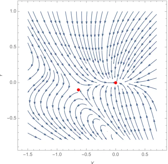
) = ( − 0.76602 . . . , +0.17501 . . .). Fig. 2.2 shows the obtained fixed points and the RG flow. The flow is very different from the one in the continuum, especially in the strong-coupling phase, i.e., the left-hand part of the figure. It is noteworthy that the sign of Y

is changed depending on the regularization.

These result show a non-universal feature of the RG flow, as one might expect.

10 CHAPTER 2. RENORMALIZATION GROUP ANALYSIS

-1.5 -1.0 -0.5 0.0 0.5

-0.5 0.0 0.5 1.0

X

Y

Figure 2.2: The same as in Fig. 2.1, but obtained with the lattice regularization with the three-point formula.

In addition to the three-point formula, we also consider the five-point formula,

| k |

→ 4 a

∑

i=1

[ sin

( k

a 2

) + 1

3 sin

( k

a

2 )]

. (2.34)

This formula has higher-order discretization errors than the three-point formula.

As we will show later, effects of the rotational symmetry breaking caused by the discretization with the three-point formula are large. Thus, we perform the same RG analysis with the five-point formula as that with the three-point formula. With this prescription, we obtain values of the constants as

θ

= 1.37619 . . . , θ

= 2

π , θ

= 15

π

, R(0) = − 0.41278 . . . . (2.35)

Here we have calculated the constants θ

and R(0) by reference to the method of

Appendix of Ref. [46]; see the Appendix of Ref. [29] for more details. With these

parameters, we find that the nontrivial fixed point is now located at (X

, Y

) =

( − 0.63338 . . . , − 0.098805 . . .). In Fig. 2.3, we show the fixed points and the RG flow.

2.2. RG FLOWS WITH THE LATTICE-REGULARIZED INTEGRALS 11

-1.5 -1.0 -0.5 0.0 0.5

-0.5 0.0 0.5 1.0

X

Y

Figure 2.3: The same as in Fig. 2.1, but obtained with the lattice regularization with the five-point formula.

The flow changes considerably from the case of the three-point formula, especially in the strong-coupling phase and becomes more similar to the flow in the continuum, as one might expect. We summarize the locations of the nontrivial fixed point in Table 2.1 as well as the constants θ

(n = 1, 3, 5) and R(0) for the RW equations in Table 2.2.

Note that the prescription discussed in this section does not produce a genuine

lattice result. On a lattice, the rotational invariance is explicitly broken so that the

notion of “partial waves” is not good. However, we just substituted the integrals

evaluated with the lattice regularization into the RG equations derived from the LS

equation for the S waves. Although the procedure is not fully consistent, the analytic

results obtained here are a very useful guide for the genuine lattice study, as shown

later.

12 CHAPTER 2. RENORMALIZATION GROUP ANALYSIS

Table 2.1: Locations of the nontrivial fixed point Regularization scheme (X

, Y

)

Sharp momentum cutoff Λ ( − 0.717691 . . . , − 0.401924 . . .) Lattice regularization with

the three-point formula ( − 0.76602 . . . , +0.17501 . . .) Lattice regularization with

the five-point formula ( − 0.63338 . . . , − 0.098805 . . .)

Table 2.2: Constants for the RW equations Regularization scheme θ

θ

θ

R(0)

Sharp momentum cutoff Λ 1 1

3 1

5 − 1

Lattice regularization with

the three-point formula 1.58796 . . . 2 π

12

π

0.754330 . . . Lattice regularization with

the five-point formula 1.37619 . . . 2 π

15

π

− 0.41278 . . .

2.3 Ground-state wave function and the ANC

In this section, we consider the stationary Schr¨ odinger equation in the continuum, before we proceed to that defined on a lattice to obtain the genuine lattice result. In momentum space, the stationary Schr¨ odinger equation for the relative motion of the two-nucleon state is given by

Eψ(p) = p

M ψ(p) +

∫

d

q (2π)

[ C

+ 4C

(

p

+ q

)]

ψ(q), (2.36) where we suppose that the wave function satisfies ψ(p) = 0 for | p | > Λ and restrict the interval of integration to be the region | q | ≤ Λ. Hereafter, we concentrate on the case with E < 0, i.e., the bound state.

The Schr¨ odinger equation can be solved in the same matter as the LS equation in Sec. 2.1. By introducing constants α and β,

α =

∫

d

q

(2π)

ψ(q), β =

∫

d

q

(2π)

q

ψ(q), (2.37) we can formally solve the Schr¨ odinger equation as

ψ(p) = − M p

+ µ

[( C

+ 4C

p

)

α + 4C

β ]

, (2.38)

where µ = √

M | E | . By multiplying Eq. (2.38) by (2π)

and p

(2π)

and integrating

2.3. GROUND-STATE WAVE FUNCTION AND THE ANC 13 over p, we obtain the system of linear equations for α and β,

( 1 − C

I

− 4C

I

− 4C

I

− C

I

− 4C

I

1 − 4C

I

) ( α β

)

= ( 0

0 )

. (2.39)

Here, we use the integrals I

defined by Eq. (2.9) but with µ = √

M | E | . Note that the coefficient matrix is the same as that appears in Eq. (2.8). The system of linear equations has a nonzero solution if the determinant D defined by Eq. (2.13) is equal to 0. This condition which corresponds to the vanishing of the denominator of the scattering amplitude determines µ, hence the energy eigenvalue E.

When the condition is satisfied, by substituting the ratio β/α, β

α = 1 − C

I

− 4C

I

4C

I

, (2.40)

into Eq. (2.38), the wave function is written as

ψ(p) = − 4M αC

+ M α [4C

µ

− (1 − 4C

I

)/I

]

p

+ µ

. (2.41)

We determine the overall normalization by the usual condition ∫

d

p/(2π)

| ψ (p) |

= 1. In the coordinate space, this function is expressed by a sum of the regularized δ function and the regularized Yukawa function. Therefore, it is natural to define the asymptotic normalization constants (ANC) as the numerator of the second term divided by 4π since the Yukawa function governs the asymptotic behavior of the coordinate-space wave function in the limit of Λ → ∞ .

By utilizing formulations explained in Sec. 2.1 and this section, We can relate the scattering length and the effective range to the binding energy and the ANC as follows.

First, we determine the coupling constants X and Y correspond to the given values of the scattering length and the effective range as a function of the cutoff Λ by solving Eqs. (2.20) and (2.21) for each value of the cutoff Λ. We then obtain the binding energy and the ANC by solving the equation D = 0 numerically.

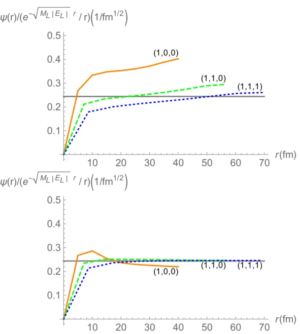
In Fig. 2.4, we show the results for the physical set of the scattering length and the effective range for the spin-triplet isospin-singlet S-wave channel, (a

, r

) = (5.42, 1.75) fm [10], corresponding to deuteron, as a function of the cutoff Λ. We see that the binding energy and the ANC are constant for a wide range of the cutoff and approximately equal to 2.19 MeV and 0.244 fm

, respectively. It is noteworthy that the obtained value of the ANC is very close to the recommended value in Ref. [10], 0.8845(8) / √

4π fm

= 0.2495(2) fm

, obtained with a completely different N N potential. (The factor √

4π comes from the normalization of the spherical harmonics.) Note that both the binding energy and the ANC vanish at Λ ≈ 57.2 MeV, cor- responding to Λ

/M ≈ 3.5 MeV in energy scale or π/Λ ≈ 10.8 fm in length scale.

Recalling that binding energy and the mean-square radius of deuteron are 2.22 MeV and 1.97 fm, we guess the behavior comes from the resolution there is too low to detect the deuteron.

The result we numerically obtained supports that we can take the binding energy

and the ANC instead of the scattering length and the effective range as the parameters

which characterize the system at low energies. Thus, to obtain the RG flow on a lattice,

we use the binding energy and the ANC as low-energy physical quantities to be fixed

in the next section.

14 CHAPTER 2. RENORMALIZATION GROUP ANALYSIS

50 100 150 200 250 300 350 400 Λ ( MeV ) 0.5

1.0 1.5 2.0 2.5 BE ( MeV )

50 100 150 200 250 300 350 400 Λ ( MeV ) 0.05

0.10 0.15 0.20 0.25 0.30

ANC  1 / fm



Figure 2.4: The binding energy (upper) and the ANC (lower) as a function of the cutoff Λ, calculated for the physical set of the scattering length and the effective range, (a

, r

) = (5.42, 1.75) fm, corresponding to deuteron [10]. The binding energy and the ANC are constant for a wide range of the cutoff and approximately equal to 2.19 MeV and 0.244 fm

, respectively. The obtained value of the ANC is very close to the recommended value in Ref. [10], 0.8845(8) / √

4π fm

= 0.2495(2) fm

,

obtained with a completely different N N potential.

2.4. NLO NEFT WITHOUT PIONS ON A LATTICE 15

2.4 NLO NEFT without pions on a lattice

In this section, we consider the Hamiltonian of the NLO NEFT without pions defined on a spatial cubic lattice to obtain a genuine lattice result. We suppose the lattice has N

sites in each directions, a finite lattice constant a, and a finite size L = N

a and is imposed the periodic boundary condition. On the lattice, the three-dimensional position vector x is replaced with na, where n is a three-dimensional vector with integer components n = (n

, n

, n

). The periodic boundary condition identifies n with n + N

e

, where e

(i = 1, 2, 3) is the unit vector in the ith direction.

The Hamiltonian of the NLO NEFT without pions in the continuum is given as H =

∫ d

x

[ N

(

− ∇

2M

)

N + C

( N

P

N )

(

N

P

N )

− C

{(

N

P

N )

(

N

P

← →

∇

N )}]

. (2.42) By performing the substitutions, H → H

a

, x → na, ∫

d

x → a

∑

n

, N (x) → N

a

, M → M

a

, C

→ C

a

, and C

→ C

a

, we obtain the dimensionless Hamiltonian on a lattice, H

, in terms of dimensionless quantities as

H

= ∑

n

[

− 1

2M

N

∇

N

+ C

(

N

P

N

)

(

N

P

N

)

− C

{(

N

P

N

)

(

N

P

← → ∇

N

)

+ +H.c.

}]

, (2.43)

where we introduced the dimensionless discretized Laplacian ∇

and ← ∇ →

. For the three-point formula, we define

∇

N

=

∑

i=1

(N

− 2N

+ N

) , (2.44)

and

N

← ∇ →

N

=

∑

i=1

[( N

− 2N

+ N

)

P

N

− (

N

− N

)

P

(N

− N

)

− (

N

− N

)

P

(N

− N

) + N

P

(N

− 2N

+ N

) ] , (2.45) so that these derivatives give the same discretized Laplacian in momentum space as we employed in Eq. (2.31) as shown shortly. Similarly, for the five-point formula, we define

∇

N

=

∑

i=1

(

− 1

12 N

+ 4

3 N

− 5

2 N

+ 4

3 N

− 1

12 N

)

, (2.46)