Variational Multiscale Finite Element Method Based on Bubble Element for Steady Advection-Diffusion Equations

(1)

富山大学人間発達科学部紀要　第 13 巻第 2 号：297−304（ 2 0 1 8 ）

学術論文

Ⅰ　Introduction

　In the framework of continuum mechanics, advection-diffusion equations are significant mathematical models describing fluid flow problems. Along with fluid mechanics, these equations are widely used in natural and engineering science problems, such as the wave propagation problem in solid mechanics, since some of the solutions for wave equations are advection-diffusion equations. In mathematical aspects, it is noted that Navier-Stokes equations can be regarded as a system of simultaneous advection-diffusion equations.

　Despite recently renewed interest in the phenomenon of advection-diffusion problems, a full understanding of it remains elusive in a framework of multiscale aspects⁽¹⁾. A complete description of advection-diffusion equations would incorporate an explanation of the computational mechanics for both subgrid

and multiscale perspectives^{(2, 3)}, as well as an understanding of stabilization aspects within stabilized finite element methods⁽⁴⁾. It is well known that the classic Galerkin finite element method lacks stability when the diffusive terms are small compared to the advective / convective terms when the cell Péclet number is higher than one^{(2, 3, 4)}. Furthermore, the classic Galerkin finite element method may produce approximate solutions with non-physical oscillations unless the subdivision width is adequately small with respect to the viscosity.

　Recently, some stabilized methods⁽⁵⁾ have been reformulated in the framework of the variational multiscale (VMS) method^{(6, 7, 8)}. In this paper, an effective VMS method is therefore proposed using a bubble element(1, 8, 9, 10) based finite element approximation with a multiscale function for advection-diffusion equations. It is noted that the resolved scale problem would be to find a solution of the VMS finite element formulation.

On the contrary, the unresolved scale problem would be likely to find the fine-scale solution captured by the L² orthogonal projection from

Variational Multiscale Finite Element Method Based on Bubble Element for Steady Advection-Diffusion Equations

Hiroshi Okumura

^＊

E-mail: okumura@itc.u-toyama.ac.jp

Abstract

　This paper presents a variational multiscale (VMS) finite element method based on the bubble element, which enables the establishing of a multiscale function to stabilize the advective-diffusive limit and the discontinuity in steady advection-diffusion problems. Furthermore, it is proved that the present VMS method is equivalent to stabilized finite element methods with the space of piecewise linear functions on elements. It is also shown that the present VMS method solves unresolvable scales under the mesh size by the Laplacian of bubble nodal values. This yields some stabilization for linear nodal values. In some numerical experiments, we show L² and H¹ error norms and the efficiencies of the present VMS method.

Keywords： Variational multiscale (VMS) method, bubble element, multiscale function, advection-diffusion equation, stabilized finite element method

※ Information Technology Center / Graduate School of Human Development, University of Toyama

(2)

The error estimation and efficiency of the present VMS method are herein shown through numerical benchmark tests to investigate the numerical accuracy and stability of the method.

Additionally, in the numerical experiments, the method’s numerical stability and effectiveness for shock capturing of the discontinuous points are discussed.

Ⅱ　Variational Multiscale Method 　We consider a bounded domain Ω⊂R^d(d=2, 3) with the boundary Γ＝∂Ω and a steady advection-diffusion equation: Find the scalar function u:Ω→R such that

　 (1)

where a∈(L^∞ (Ω) )^d,υand f∈L^∞ (Ω) the advection velocity vector, viscosity, and source function, respectively. Parenthetically, we note that the divergence-free condition ∇⋅a=0 is not imposed on the equation (1). For simplicity, the Dirichlet boundary condition is imposed on the partial differential equation (1).

　Let functional spaces ν=H¹ (Ω), 0 L = (L² (Ω))^d of the conventional Variational Multiscale (VMS) method for the advection-diffusion equation (1) yield the following coupled variational problem

(2, 3, 7) : Find u∈V, g∈L such that

(2) with a bilinear form

(3) where is an arbitrary function νadd, which will be discussed further below. We herein call this function νadd multiscale function.

　For the finite element approximation of this variational problem (2), let Th be the regular triangulation of the domain Ω. We define the mesh parameter (i.e., mesh size) h=max(diam(K)) as the maximum diameter for any element K∈

Th. For the VMS finite element formulation we propose, we choose the bubble element space Vh,

element space V₁ and the bubble function space B(K).

(4) where ϕK∈B(K) is the bubble function with compact support defined in each element K∈

Th. It is remarkable that the bubble functions ϕK is zero on the element boundary ∂K, which is usually defined by using piecewise high-order polynomials in K∈Th (9). Incidentally, the bubble nodal value is denoted by ubK. Furthermore, we choose the piecewise constant vector space R0d

for the approximation of the vector subspace L in the second problem of the coupled variational problem (2).

(5) 　We approximate the multiscale variational problem (2) by using the bubble element (4) and the piecewise constant vector (5). We then have a fully discretized problem(2, 3, 7, 8) : Find, Gh∈R0d such that

(6) 　The second equation of (6) states that Gh=Ph∇ uh, where Ph is the L²-orthogonal projection from

∇Vh into R0d. We also choose Ph based on the one- point Gauss integral Ph:∇Vh→R0d such that

(7) where qbK is the barycenter point of each triangular element K∈Th. Then, we obtain

(8) since Ph∇vh∈R0d, where I is an identity operator.

　Besides the derivation of equation (8), the relationship of Ph∇u1=∇u1 and Ph∇v1=∇v1 holds in the piecewise linear element. Furthermore, the condition of orthogonality (10, 12, 13) between piecewise linear functions and the bubbles yields

(9) where (⋅, ⋅)K denotes the integration in element K.

(3)

Variational Multiscale Finite Element Method Based on Bubble Element for Steady Advection-Diffusion Equations

　Hence, the fully discretized problem (6) of the coupled variational multiscale problem (2) for the advection-diffusion equation is equivalent to the following discretized problem:

(10)

　Remark 1. It is obvious that the term (I-Ph)∇

uh shows a small fluctuation with respect to ∇ uh. It is also safe to predict that the second term of the left-hand side in (10) denotes the Laplacian, which acts as stabilization for unresolvable scales under the mesh size h.

　We focus on the second term of the left-hand side in the discretized problem (10). Suppose that the multiscale function νadd is constant in K.

Hence, the following relationship holds as

(11)

　Thus, the discretized problem (10) can be rewritten:

(12) 　Furthermore, the classic bubble function(9, 10, 12, 13) could be chosen. It is defined by the product of area / volume coordinate λi (i=1,…, d+1)

(13) where i denotes the vertices of triangular / tetrahedral element K shown in Figure 1 (d=2).

In detail, (12) can be rewritten as

(14) since the L²-orthogonal projection of the bubble function (13) yields

In addition, the approximate equation (14), which can be derived by the approach of the present VMS finite element formulation, seems to be approximately equivalent to the term υ

add (∇ub,∇vb)K added to the Bubnov-Galerkin method proposed by Guermond (1999)⁽⁵⁾. However, a full understanding and an evaluation of the multiscale function is elusive in the studies^{(5, 7, 8)}. 　Remark 2. The possibility exists that residual-free bubbles (RFB)⁽¹¹⁾ and P-scaled bubble functions^{(12, 13)} could be employed as candidates for a bubble function. However, it is noted that those special bubble functions cannot be applied to the present VMS finite element approximations (10)-(12) because those functions have a singular point on the barycenter of each triangular / tetrahedral element.

　In returning to (10), we evaluate the multiscale function υadd, as mentioned above. We consider static condensation procedure of the bubble functions. Let us write the solution uh of the VMS formulation (10) as

(15) where u1∈V1, ubK is the bubble nodal value, and ϕK∈B(K) is the bubble function (13).

　Let vh=ϕK in (10). Moreover, assuming f and a to be the piecewise constant in K, we can obtain the bubble nodal value as

(16) where ‖ ⋅ ‖K denotes the L² (K) norm.

　Let us now consider vh=v1 in (10). Then, we can obtain the P1 finite element approximation by means of the static condensation procedure eliminating the bubble nodal values: Find u1∈V1, such that

Figure 1. A classical bubble function φK defined on triangle element K∈Th (d=2)

(4)

(17) where τK is the stabilization parameter of the VMS finite element formulation based on the bubble element.

(18) where hK is the diameter of K.

　Remark 3. It can be proved that the finite element approximate equation (17) of the VMS formulation is coercive over V1 under the assumptions that V1 is the space of piecewise linear functions on triangles or tetrahedral elements K, that the triangulation τh is regular, and that this regularity is uniform as h→0 by way of the analogy of the stabilized finite element method, such as the streamline-upwind / Petrov-Galerkin (SUPG) method⁽¹⁴⁾.

　Remark 4. For the advection-diffusion problem (1), it is remarkable that the finite element approximate equation of the present VMS finite element method based on the bubble element is equivalent to stabilized finite element methods and the SUPG method with linear elements, in which the stabilization effect, including the Laplacian upwind tensor of the advection velocity field, uses P1 finite element approximation. The magnitude of the stabilization parameter τK

of (18) is determined by the shape of the bubble function ϕK and the multiscale function νadd. 　In contrast, the stabilization parameter τSUPG

of the SUPG method⁽¹⁴⁾ is given as follows:

(19)

Therefore, the relationship of (18) and (19) is linked and engenders the criteria of the multiscale function

(20) 　Remark 5. Choosing the classical bubble

the bubble degree of freedom in the finite element approximate equation (12) can be obtained simply as

(21) since Ph∇ϕK=0 obviously.

Ⅲ　Numerical Experiments

　In this section, we estimate L² and H¹ error norms of the present VMS finite element method for examples with analytical solutions.

Furthermore, we show the numerical results and compare the numerical performance of the present method with the multiscale function to established techniques.

1. Error estimation with analytical solution 　In the convergence analysis, we consider a simple advection-diffusion problem on a unit square domain Ω=(0,1)×(0,1) that can be analytically solved. As shown in Figure 2 for the problem statement, we consider the domain subjected to the specified boundary conditions.

There are no distributed sources f, and the advection velocity is a=(a1, a2)=(0,1) in Ω.

Then, the problem gives the exact solution:

(22) where

Figure 2. Problem statement of an example with an analytical solution

(5)

(23)

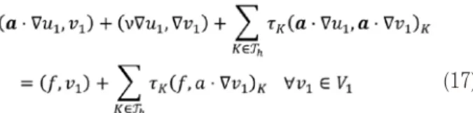
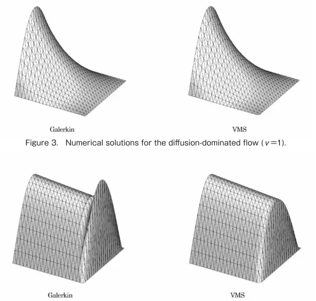
　We consider two different values for the viscosity ν=1 and ν=10^-2, so that we can compare the results of the conventional Galerkin method⁽⁹⁾ based on bubble element using the classical bubble function (13) and those of the present VMS approach. The numerical solutions are shown in Figure 3 for ν=1, and in Figure 4 for ν=10^-2.

　In every case of the computations by the present VMS finite element method, smooth numerical solutions are obtained. On the other hand, it is observed that the numerical solution of the classical Galerkin method provides non-

physical oscillations along the boundary layer for the advection-dominated case, ν=10^-2. As the result, the present VMS exhibits the best performance on this problem. We note that the version of VMS implemented herein is designed for the advection limit, whereas this problem contains diffusion-dominated regions.

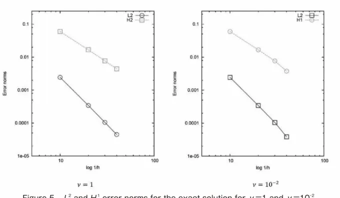
　As shown in Figure 5, we additionally obtain second-order convergence in the L² error norm and first order convergence in the H¹ error norm when ν=1 and ν=10^-2, respectively. However, for ν=10^-2, the convergence rate slightly increases for both of them. Moreover, the present VMS finite element method is more accurate than the Galerkin method in the advection-dominated flow problems on account of the effect of the multiscale function νadd.

Figure 4.　Numerical solutions for the diffusion-dominated flow (ν=10^-2).

Figure 3.　Numerical solutions for the diffusion-dominated flow (ν=1).

(6)

Figure 7.　Regular triangulations Th of the domain Ω Figure 6.　Problem statement of advection skew to the mesh

(7)

2. Advection skew to the mesh

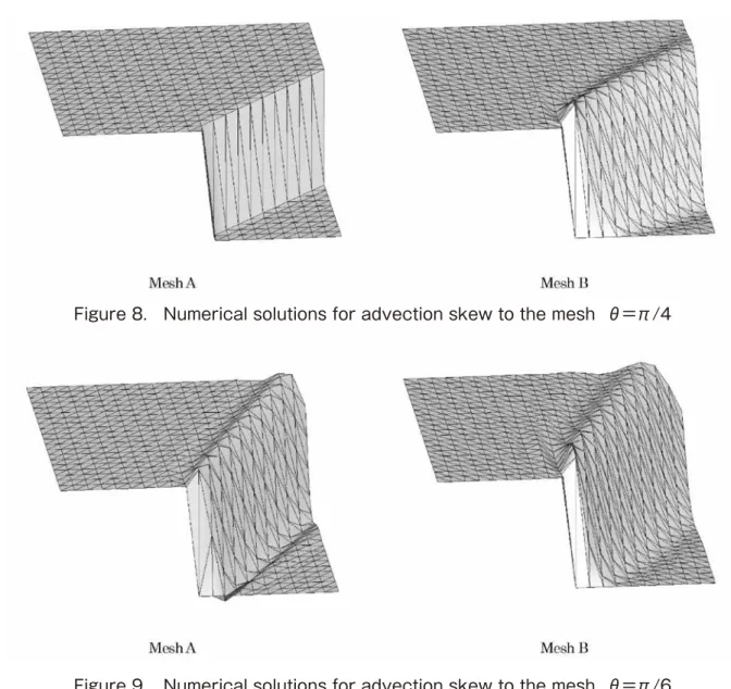
　We consider a modified problem so that a discontinuity exists in the inflow Dirichlet condition at x=(0.5, 0) with the homogeneous Neumann outflow condition, as shown in Figure 6. This is a popular problem involving oblique shock and discontinuous points. The discontinuity is propagated into the domain, thereby creating an internal layer. Here, ν

=10^-4. Using two uniform triangular meshes A and B (Figure 7), the problem is solved at θ=

π/4 and θ=π/6 are shown in Figures 8 and 9. These numerical results indicate that the discontinuity shock is captured within a few elements for all the meshes. It is remarkable that the solutions demonstrate some improvement over the Galerkin method. Furthermore, θ=π

/4 on mesh A provides the exact solution and exhibits the performance for these problems with the discontinuities, particularly when the flow is along the element diagonals.

Ⅳ　Conclusion

　The proposed VMS finite element method with the multiscale function defined on the bubble degrees of freedom was shown to be an effective stabilized finite element method for the advection diffusion equation. It can compute flow problems with the advective limit and the discontinuous points contain diffusion-dominated regions. It was additionally shown that the error estimation of the VMS method in which the second-order convergence in the L² error norm and the first- Figure 9.　Numerical solutions for advection skew to the mesh θ=π/6

Figure 8.　Numerical solutions for advection skew to the mesh θ=π/4

(8)

both advective and diffusive limits existed in the numerical experiment.

Acknowledgement

　This work was supported by JSPS KAKENHI, Grant Number JP16K13734.

References

(1) T. J. R. Hughes: Multiscale phenomena:

Green's functions, the Dirichlet-to-Neumann formulation, subgrid scale models, bubbles, and the origin of the stabilizaed formulation，

Computer Methods in Applied Mechanics and Engineering，Vol.127, pp.387-401, 1995.

(2) R. Codina: On stabilized finite element methods for linear systems of convection- diffusion-reaction equations, Computer M e t h o d s i n A p p l i e d M e c h a n i c s a n d Engineering, Vol.188, pp.61-82, 2000.

(3) R. Codina: Stabilization of incompressibility and convection through orthogonal sub-scales in finite element methods, Computer Methods in Applied Mechanics and Engineering, Vol.190, pp.1579-1599, 2000.

(4) L. P. Franca and T. J. R. Hughes:

Convergence analysis of Galerkin least-squares methods for advective-diffusive forms of the Stokes and incompressible Navier-Stokes equations, Computer Methods in Applied Mechanics and Engineering, Vol.105, pp.285- 298, 1993.

(5) J. L. Guermond: Stabilization of Galerkin approximations of transport equations by subgrid modeling, M2AN Mathematical Modelling and Numerical Analysis, Vol.33, pp.1293-1316, 1999.

(6) T. J. R. Hughes, G. R. Feijóo, L. Mazzei and J.

B. Quincy: The variational multiscale method - a paradigm for computational mechanics, Vol.166, pp.3-24, 1998.

(7) V. John, S. Kaya and W. Layton: A two-level

dominated convection-diffusion equations, Computer Methods in Applied Mechanics and Engineering, Vol.195, pp.4594-4603, 2006.

(8) L. Song, Y. Hou and H. Zheng: A variational multiscale method based on bubble functions for convection-dominated convection- diffusion equations, Applied Mathematics and Computation, Vol.217, pp.2226-2237, 2010.

(9) D. Boffi, F. Brezzi and M. Fortin: Mixed finite element methods and applications, Springer, Berlin Heidelberg, 2013.

(10) H. Okumura and M. Kawahara: A new stable bubble element for incompressible fluid flow based on a mixed Petrov-Galerkin finite element formulation, IJCFD, Vol.17 (4), pp.275- 282, 2003.

(11) F. Brezzi, L. P. Franca, T J. R. Hughes and A. Russo: b=∫ɡ, Computer Methods in Applied Mechanics and Engineering , Vol.145, 329-339, 1997.

(12) J. C. Simo, F. Armero and C. Taylor:

Galerkin finite element methods with bubble for advection dominated incompressible Navier- Stokes, International Journal for Numerical Methods in Engineering, Vol.38, pp. 1475-1509, 1995.

(13) T. Yamada: A bubble element for the compressible Euler equations, IJCFD, Vol.9, pp.273-283, 1998.

(14) A. N. Brooks and T. J. R. Hughes: Streamline Upwind/Petrov-Galerkin formulation for convection dominated flows with Navier-Stokes equations, Computer Methods in Applied Mechanics and Engineering, Vol.32, pp.199-259, 1994.

（2018年10月22日受付）

（2018年12月19日受理）