An ec onom
et r i c anal ys i s of unc onvent i onal
m
onet ar y pol i c y : t he c as es of J apan and
U
ni t ed St at es
著者
Shi bat a Ts ubas a, Kos aka H
i r oyuki
権利
Copyr i ght s 日本貿易振興機構(ジェトロ)アジア
経済研究所 / I ns t i t ut e of D
evel opi ng
Ec onom
i es , J apan Ext er nal Tr ade O
r gani z at i on
( I D
E- J ETRO
) ht t p: / / w
w
w
. i de. go. j p
j our nal or
publ i c at i on t i t l e
I D
E D
i s c us s i on Paper
vol um
e
704
page r ange
1- 36
year
2018- 03
研究会名
新しいグローバル・モデルの開発とその応用
INSTITUTE OF DEVELOPING ECONOMIES
IDE Discussion Papers are preliminary materials circulated
to stimulate discussions and critical comments
* Institute of Developing Economies, Japan. Email: [email protected]
**
Keio University, Japan. Email: [email protected]
IDE DISCUSSION PAPER No. 704
An Econometric Analysis of
Unconventional Monetary Policy:
The Cases of Japan and United States
Tsubasa SHIBATA* and Hiroyuki KOSAKA**
The Institute of Developing Economies (IDE) is a semigovernmental,
nonpartisan, nonprofit research institute, founded in 1958. The Institute
merged with the Japan External Trade Organization (JETRO) on July 1, 1998.
The Institute conducts basic and comprehensive studies on economic and
related affairs in all developing countries and regions, including Asia, the
Middle East, Africa, Latin America, Oceania, and Eastern Europe.
The views expressed in this publication are those of the author(s). Publication does not imply endorsement by the Institute of Developing Economies of any of the views expressed within.
INSTITUTE OF DEVELOPING ECONOMIES (IDE), JETRO
3-2-2, WAKABA,MIHAMA-KU,CHIBA-SHI
CHIBA 261-8545, JAPAN
©2018 by Institute of Developing Economies, JETRO
1
An Econometric Analysis of Unconventional Monetary Policy:
The Cases of Japan and United States
Tsubasa Shibata
†Hiroyuki Kosaka
‡March 14, 2018
Abstract
In the wake of financial crisis, the use by major advanced countries of unconventional
monetary policies, such as credit easing (CE) by central banks toward depository banks
as well as quantitative easing (QE), is not without controversy. While QE increases the
liability side of the central bank's balance sheet by expanding the monetary base, the new
phase of CE policy enlarges the asset side by purchasing different types of credit in order
to get credit markets functioning. Nevertheless, many studies have not taken this
important difference in policy into account. They have shed light on mechanisms of the
determination of interest rate but precluded any endogenous movement of items in the
balance sheets of central banks. Instead, this paper attempts to construct a financial model,
linked to a macro-econometric model, which reflects the central bank’s balance sheet.
The two linked models provide a better guide to explaining how a central bank’s monetary
policy generates impacts on the real economy via depository banks. By undertaking a
comparative assessment of the cases of Japan and the USA, this study conducts scenario
simulation using the two linked models. It thereby offers an alternative solution to current
monetary policy that aims to tackle the problem of deflation.
Keywords: Unconventional monetary policy, financial market, macro-econometric model.
JEL Codes: E10, E17, E44, E52
† Institute of Developing Economies, Japan. Email: [email protected]
2
1.
Introduction
The global financial crisis in 2008 nearly sent the world economy into a depression. To forestall such a calamitous event, central banks and monetary authorities in major advanced economies, such as Japan, USA, European Union, and Britain, implemented policies to lower their interest rates so drastically as to approximate a zero lower bound point. In principle, when the interest rate is lower zero bound, the economy is assumed to fall into a liquidity trap (Hicks, 1937). Despite these bold, if desperate, monetary policies, many economies could not avoid or overcome severe downturns. It appeared that the monetary policy tool of simply lowering interest rates, based on traditional monetary theory, was in practice not sufficiently effective for achieving the objectives of central banks. Under the circumstances of severely ailing money markets, the central banks were compelled to adopt unconventional instruments to expand the overall money supply.
By definition, an unconventional monetary policy can be any policy introduced by a central bank in a situation where the policy interest rate is lower zero bound or nearly so (Miyao, 2006). Some years before the crisis developed, Bernanke and Reinhart (2004) and Bernanke et al. (2004) suggested that central banks had several options in the use of unconventional monetary policy even in situations of policy interest rate lower bound. Specifically, certain policies could aim for credit easing (CE) by purchasing private sector assets, such as commercial paper and residential asset-backed securities, and/or aim for quantitative easing (QE) by large-scale purchases of government securities. Indeed, the USA’s Federal Reserve System (Fed) carried out large-scale purchases of mortgage-backed securities while the Bank of Japan (BOJ) bought index-linked exchange-traded funds (ETF) and Japanese real estate investment trusts (J-REIT). In short, some central banks chose to expand private debts over a wider range as a form of monetary policy instrument in order to keep many credit markets functioning.
How do such monetary policies affect financial markets and the real economy? How should we appraise and evaluate these central banks’ decisions? Is it feasible to overcome deflation with unconventional monetary measures?
3
preclude any endogenous movement of items within a central bank’s balance sheet. A notable exception is the study by Cúrdia and Woodford (2011) which, using the New Keynesian model, includes the central bank’s balance sheet in their analysis of the effectiveness of monetary policy. Most other Keynesian models, which accept that the long-term interest rate is determined by money supply, have not dealt with any aspect of a central bank’s balance sheet. In fact, few studies have shown interest in the balance sheets of central banks.
As a rule, however, each identical relations between the balance sheets of central banks and those of depository banks should be retained in analysis in order to trace the transmission channels by which a purchase of private assets affects the real economy through the financial markets. For this reason, this paper attempts to construct a financial model, linked to a macro-econometric model, which reflects the central bank’s balance sheet. In the opinion of Shibata and Kosaka, the two linked models provide a better guide to explaining how a central bank’s monetary policy generates impacts on the real economy via depository banks. Here, by undertaking a comparative assessment of the cases of Japan and the USA, our study conducts scenario simulation in the use of two linked models. The study thereby offers an alternative solution to current monetary policy that aims to tackle the problem of deflation.
4
2.
Analytical Framework of Financial/Macroeconometric Model
In this section, we will illustrate the theoretical framework of our financial model for analyzing unconventional monetary policy. The structure of our model consists of two sectors: the monetary sector and the real sector. The economic activities in the financial sector are composed of a central bank, depository institutions, and the private sector (i.e., households and industries). The decision making of the central bank and depository institutions as well as interest rates will mainly be discussed in the basic framework for the financial model in this section, following the basic ideas outlined by Klein and Krelle (1983) and Sadahiro (1992). The economic activities of the private sector will be explained by the traditional and simple Klein’s skeleton model (1983), which is presented in Appendix A.
2.1.
Optimal Control Monetary Policy by Central Bank
Under current monetary policy, the central bank sets the policy interest rate close to zero lower bound and increases liquidity in the financial system by purchasing government bonds, corporate bonds, and asset-backed securities, which encourages commercial banks to provide loans and promote the real economy. We assume the objective functions of monetary policymakers based on each credit.
2.1.1. Determining Monetary Instruments
a) Government Treasury Bonds – Unconventional Monetary Policy
First, we consider the monetary policy instrument of a government securities purchase. It is supposed that central banks attempt to affect long-term interest rates by purchasing large scale government securities. The statement of policy objectives could be expressed by the social welfare function formed by the quadratic loss form (Pissarides, 1972; Friedlaender, 1973; Chow, 1975) as follows:
, = � ( ,� − ∗,� ) + ( , − ∗, ) (3.1)
where , denotes the amount of domestic government treasury bonds purchased by the nth
country’s central bank and ,� shows that country’s interest rate (long-term interest rate). ,� is
a policy target variable and , is a policy instrument. The asterisk (*) indicates the desired level
5
b) Other Credit Offering – at New Phase of Unconventional Monetary Policy
Next, consider another monetary policy instrument: buying other private assets. Purchasing asset-backed securities equities and private sector debts is assumed to affect stock prices and promote private consumption and investment. We formulate the policy objectives of central bank as:
= � − ∗ + � − ∗ + � − ∗ + − ∗ (3.2)
where and show household consumption and private investment in current prices,
respectively, and represents the stock market price index, which refers to policy target variables. as the policy instrument denotes the amount of asset-backed securities purchased.
Here, we consider in the context of the United States and Japan. Although the US Federal
Reserve does not have the ability to directly affect mortgage rates, quantitative easing and credit easing indirectly impact on the stock market through the purchase of government securities and mortgage-backed securities (MBS). Likewise, the Bank of Japan has been increasing its domestic equity holdings by purchasing index-linked exchange-traded funds (ETF) and Japanese real estate investment trusts (J-REIT), which eventually leads to some impact on the stock markets. The model would be required to reflect these realities.
First, as for United States, purchases of private assets would be represented as:
, = � − ∗ + � − ∗ + � ( , − ∗, )
+( , − ∗ , )
(3.3)
where , corresponds to the Dow Jones Industrial Average and , means the amount of
MBS purchased.
Next, in the case of Japan, the Bank of Japan continues to purchase ETF and J-REIT, attempting
to exert a positive impact on stock markets and other asset markets. Therefore, , should be
divided into two parts: for EFT and for J-REIT. Moreover, since there are two types of
ETF, would be further divided into two more parts: , for ETF tracking the Nikkei 225
Index and , tracking Tokyo Stock Price Index.
Firstly, as for ETF, it is seen that there is the same trend between the accumulation of EFT holdings by the Bank of Japan and domestic stock price indices. The Bank of Japan holding ETF should theoretically support stock prices, which might lead to increased consumption and boost private investment. Taking these factors into consideration, the policymakers’ policy objective with regard to
6
, = � ( − ∗ ) + � ( − ∗ )
+� ( , − ∗ , ) + � ( �, − ∗ �, )
+( , − ∗ , ) + ( , − ∗ , )
(3.4)
where is private residential investment in current prices, , represents the Nikkei
Stock Price Index, �, denotes the Tokyo Stock Price Index. Concerning policy target variables.
, and , is the amount of buying of ETF tracking the Nikkei 225 Index and the Tokyo
Stock Price Index, respectively.
Next, considering J-REIT and the policy target variable , , we can also see the same
relation between the holdings of J-REIT and the Tokyo Stock Exchange REIT Index. Purchases of real estate would impact on private residential and non-residential investment. The policy objective of the
Bank of Japan regarding , is described as:
, = � ( − ∗ ) + � ( − ∗ )
+� ( , − ∗ , ) + ( , − ∗ , )
(3.5)
where denotes non-residential investment in current prices and , represents the Tokyo
Stock Exchange REIT Index.
2.1.2. Deriving Optimal Policy Instruments
We can derive the optimal policy function, namely the policy reaction function, resulting from the central bank’s attempt to minimize the difference between the actual and desired level. Thus, we
minimize each of the above equations by the corresponding policy instruments , , ,
, , , and , and rearrange them. The following policy reaction function
toward (3.1) are obtained as:
, = ∗, − � ( ,� − ∗,� )�� ,�
, (3.6)
7
, = ∗ , − � − ∗ ��
,
−� − ∗ �
� , − � ( , − ,
∗ ) �
� ,
(3.7)
While, the policy reaction functions about purchasing asset-backed securities ETF and J-REIT by the Bank of Japan are shown as:
, = ∗ , − � ( − ∗ )��
, − � ( −
∗ ) �
� ,
−� ( , − ∗ , )�� ,
,
(3.8)
, = ∗ , − � ( − ∗ )��
, − � ( −
∗ ) �
� ,
−� ( �, − ∗ �, )��
,
(3.9)
, = ∗ , − � ( − ∗)��
, − � ( −
∗ ) �
� ,
−� ( , − ∗ , ) �� ,
,
(3.10)
These policy reaction function is estimated by the optimal-control technique. When attempting to decide current period policy, central banks are assumed to respond to movement some important economic variables over time. The optimal control method can reflect them.
2.2.
Optimal Behavior of Private Depository institutions
In this subsection, we consider the decision making of depository institutions, namely, optimal loans of depository institutions from the central bank and their optimal lending to the private sector.
2.2.1. Determining Optimal Loans from the Central Bank
8
and the interest they receive on loans. When depository institutions are assumed to receive loans from central banks at discount rates, financing received from central banks is utilized for short-term liquidity needs for borrowing for financial institutions. When reflecting these realities, the problem of commercial banks can be formalized by short-term profit maximization as:
� = − � − ∗ − � −
+ ∗ − + ∗ − ∗ +
(3.11)
where denotes borrowings of depository banks from the central bank, ∗ indicates the targeted
level of , shows loans from depository banks to consumers and business, and is the
primary deposit. is the short-term interest rate, is the discount rate, is the depository rate,
and is the lending rate.
The quadratic loss function in the upper line of equation (3.11) represents a proportional relation between the borrowing of commercial banks from a central bank and the lending of commercial banks to the private sector. It is supposed that the more money supplied to commercial banks by the central bank, the more banks are encouraged to lend to the private sector (and vice versa).
The terms in the lower line of equation (3.11) describe the profit of commercial banks.
implies financing received from central banks and intends that money provided by central banks
is invested in short-term liquidity needs by financial institutions. Thus, revenue is represented by
and , whilst the cost is shown by , , and .
We consider the first order conditions for this problem with respect to . In this process, the
term of partial derivatives � ⁄� is assumed to represent conjectural variations placed by � . We
can yield the following equation.
=�
∗ − � − � + ∗ − + �∗ − �∗
� − � − � (3.12)
Here, by replacing ∗= and = � − � − � , the optimal borrowing of depository
banks from central bank is shown as follows:
=� ∗ −� − � + − +� − � (3.13)
9
2.2.2. Determining Optimal Lending to Private Sectors
This section describes the optimal lending of depository banks (commercial banks) to the private sector, which implies a theory of money creation—the so-called “money multiplier”—that money is created via banks making loans. The central bank is assumed to affect the quantity of money in circulation. The increase of money supply is assumed to trigger the creation of reserves and growth in the broader monetary aggregate.
It is assumed that depository banks attempt to make profits by lending money to customers. Meanwhile, depository banks are forced to follow tight regulations for risk management, which means that bank lending is constrained. Hence, it is assumed that the depository banks attempt to determine the optimal lending to maximize profit over the long-term as:
� = − � − − � { − + }
− � − � � + ∗ − ∗ +
(3.14)
where denotes loans from commercial banks to consumers and business. � is total assets of
commercial banks, which implies capital adequacy ratio 8 %, namely Basel regulation. With an
assumption of � ∗⁄� = , the optimal condition is as:
��
� = −� − − � − � { − + }
−� − � � + − =
(3.15)
Here, we rewrite this equation for ∗= . The term of partial derivatives � ⁄� is regarded as
conjectural variations, and placed by � . The optimal lending is derived as:
=� − � +� + +� � � + −
= − � � + � + �
(3.16)
The second term + represents quantitative easing and credit easing by purchasing treasury
securities and other private assets. The unconventional monetary policy aims to drive lending by
depository banks to public through + . It is thought that central banks attempt to impact the
10
2.3.
Identical Relation of Money Supply
According to Klein and Krelle (1983), money supply is directly defined by credit creation multiplier as follows:
= (3.17)
where is money supply, is reserve money and is credit multiplier. However, in order to
grasp more detailed process of money creation, we modify this original model as:
= � , (3.18)
The interest rate of lending loans related to is attempted to be endogenized in the next sub-section.
2.4.
Determination of Interest Rates
i. Short-Term Interest Rate
The policy interest rate is the most important interest rate in the economy, as it is the basis for all other short-term interest rates. The policy interest rate is charged in interbank transactions. Depository banks charge their customers the prime rate based on the policy interest rate. Therefore, the policy interest rate affects other interests including other short-term interest rates, lending rates, and deposit rates. Thus, the short-term interest is assumed to be explained by the policy interest rate and the interest rate of reserve deposit requirement as:
= � , (3.19)
where denotes the monetary policy interest rate and is the interest rate of reserve deposit
requirement. The policy interest rate corresponds to the overnight call rate in Japan and the Federal Fund Rate (FFR) in United States.
ii. Discount Rate
The discount rate is one of the policy tools of central bank. Since the movement of discount rate is supposed to be closely related to policy interest rate, we set as:
= � (3.20)
11
iii. Lending Rate
It is assumed that the interest rate of lending from commercial banks to public has basically be in a same response to the short-term interest rate. We set the following equation.
= � (3.21)
iv. Long-Term Interest Rate
The long-term interest rate is thought to be based on the point of equilibrium in the money market.
Assuming = , the equilibrium of the money market is represented as:
= − � + (3.22)
where is real total output. This is the real money demand function. In short, holding money is an alternative to holding bonds. The decision for an individual’s portfolio would be divided into money and bonds. Namely, the motivation for the determination of portfolio choice depends on interest rates.
We introduce the investor’s portfolio choice theory following Markowitz1 . Thus, the real demand
function can be redefined as:
= = + + − − ⋯ −
= + + − − ⋯ −
(3.23)
Rearranging (3.23) for � , we obtain as:
� = − + (3.24)
Additionally, the long-term interest rate is in a practical arbitrage relation with the short-term market and to the international bond market, and in a correlation to the domestic stock market. Taking this into consideration, the long-term interest rate can be extended as follows:
� = − + + + � − (3.25)
where � denotes the interest rate of treasury securities and represents price to earnings ratio
in the domestic stock market.
12
2.5.
Description of the Stock Market
As historical experience of the bubble economy in Japan suggests, the financial market is interrelated with the stock market. Therefore, we make the transmission channel between stock market and financial market as:
= �(� − , ,− ) (3.26)
where denotes the representative price index in the stock market. This variable corresponds to the Nikkei Stock Average in Japan and to the Dow Jones Industrial Average in the United States.
Additionally, the stock price variation is assumed to affect consumption and investment. Taking this into consideration, we endogenize the price to earnings ratio (P/E ratio) that reflects the performance of the stock market.
= , − (3.27)
The P/E ratio is historically explained by real total output and . As mentioned above,
is determined macro economy block (See Appendix. A)
13
3.
Empirical Analysis
3.1.
Data
We employ several data sources to investigate to construct the empirical model for analysis of current monetary policy about the case of Japan and the United States.
For constructing a Japanese macro econometric model, we mainly use the quarterly National Accounts Statistics of each countries. The Source of U.S. economic statistics is published by the U.S. Bureau of Economic Analysis (BEA), agency of Department of Commerce. The Japanese National Economic Accounting is from Cabinet Office, Government of Japan. We can get these data from first quarter of 1980 to the third quarter 2016.
Also, as for building to model for a monetary sector, we utilize the data from central banks: the Bank of Japan and the Board of Governors of Federal Reserve System. We use the data like balance sheet of central bank, some kinds of interest rates (lending a loan, depository, and short-term etc.) and stock market data. The data source of long-term interest rate, 10-year government bond rate in Japan, is from the Ministry of Finance, Japan. And, 10-year treasury long-term rate data in the United States is from the U.S. Department of The Treasury.
3.2.
Estimated Results and Final Test
3.2.1. Estimated Results
We estimate the stochastic equations of the model for the monetary sector and the macroeconomic sector of Japan and the United States respectively. The sample period of this model is from the first quarter 2008 to the third quarter 2016, that is, the time period for the implementation of the unconventional monetary policy since the global financial crisis in 2008. We applied ordinary least squares. Here, we would show the several estimation results about crucial variables. The summary is
as follows2.
(i) Optimal Bank Loans from the Central Bank
Table 1 represents the estimated results of optimal loans of depository banks from the central
bank in Japan3 . This model employs approximations. From the estimated results, we see that the
relation among interest rates affects the lending from central banks. We conclude that the calculations are acceptable.
2 The estimation result of macroeconomic sector would be represented in Appendix A.
14
Table 1. Optimal Loans of Depository Banks from Central Bank in Japan: Sample 2000q2-2017q1
Explanatory Variables Coefficient S.E.
Loans to Depository Banks 0.061 0.061406
(Short-Term Interest Rate (-2)-Discount Rate (-2))/Short-Term Interest Rate (-1) -127.017 -127.0166
Deposit Rate(-2) / Short-Term Interest Rate (-1) -1830.134 -1830.134
Dummy from 2000q1 to 2017q4 -199947.5*** -199947.5
AR (1) 0.911*** 0.911391
Constant 1847.530*** 466136.7
Observation 66
Adj. R-squared 0.964
Note: Adj. R-Squared is adjusted R-squared. “S.E.” indicates robust standard errors. ***, **, and * represent significance at the 1%, 5%, and 10% levels, respectively.
(ii) Optimal Loans to Banks Private Sectors
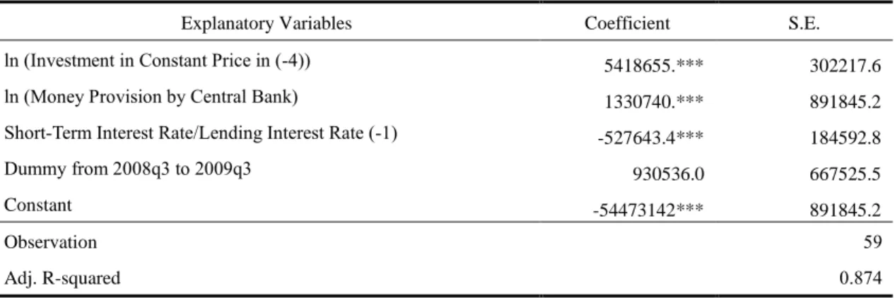
Table 2 and Table 3 represent the estimated results of optimal loans of depository banks to the private sector (i.e., consumers and industries) in Japan and the United States, respectively. Statistics show that prices are well estimated. Both tables clearly show that money provision by central banks affects depository banks’ lending to customers. This effect is most obvious in the case of the United States. At the same time, we can see a relation between lending to customers and investment, that is, a relation between monetary markets and the real economy. It is supposed that there is an impact of unconventional monetary policy on the real economy. We conclude that these results are largely acceptable.
Table 2. Optimal Lending of Depository Banks to Private Sectors in Japan: Sample 2003q1-2017q1
Explanatory Variables Coefficient S.E.
ln (Investment in Constant Price in (-4)) 0.088461 0.078
ln (Money Provision by Central Bank(-2)) 0.051210* 0.023
Short-Term Interest Rate/Lending Interest Rate (-1) -0.028976 0.035
Dummy from 2008q4 to 2009q1 0.017072*** 0.004
AR(1) 0.978545*** 0.027
Constant 13.56766*** 0.814
Observation 57
Adj. R-squared 0.978
15
Table 3. Optimal Lending of Depository Banks to Private sectors in the U.S.: Sample 2003q1-2017q1
Explanatory Variables Coefficient S.E.
ln (Investment in Constant Price in (-4)) 5418655.*** 302217.6
ln (Money Provision by Central Bank) 1330740.*** 891845.2
Short-Term Interest Rate/Lending Interest Rate (-1) -527643.4*** 184592.8
Dummy from 2008q3 to 2009q3 930536.0 667525.5
Constant -54473142*** 891845.2
Observation 59
Adj. R-squared 0.874
Note: Adj. R-Squared is adjusted R-squared. “S.E.” indicates robust standard errors. ***, **, and * represent significance at the 1%, 5%, and 10% levels, respectively.
(iii) Long-Term Interest Rate
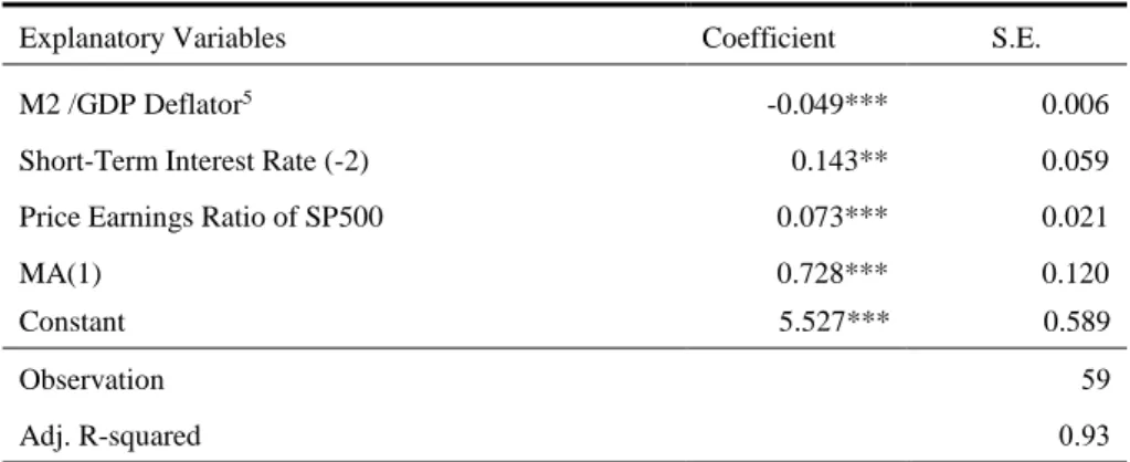
Central banks purchase government securities and other securities from markets by quantitative easing (QE) in unconventional monetary policy in order to increase money provision and lower interest rates. Also, quantitative easing (QE) in unconventional monetary policy is conducted to promote lending and liquidity through the increase in central bank reserves on commercial banks’ balance sheets. The aim of these policies is to boost stock market performance and reduce long and medium term interest rates on government securities and mortgage bonds. Tables 4 and 5 demonstrate that the money provision by the central bank, the P/E ratio in the stock market, and short-term interest rate affect the long-term interest rate.
Table 4. 10-Year Government Bond Rate in Japan: Sample 2000q2-2017q1
Explanatory Variables Coefficient S.E.
M2 /GDP Deflator4
-0.367*** 0.111
Short-Term Interest Rate 0.564 0.431
Price Earnings Ratio 0.402*** 0.211
AR (1) 0.854*** 0.058
Constant 3.710*** 0.817
Observation 68
Adj. R-squared 0.92
Note: Adj. R-Squared is adjusted R-squared. “S.E.” indicates robust standard errors. ***, **, and * represent significance at the 1%, 5%, and 10% levels, respectively.
16
Table 5. 10-Year Treasury Yield Rate in the U.S.: Sample 2003q1-2017q3
Explanatory Variables Coefficient S.E.
M2 /GDP Deflator5 -0.049*** 0.006
Short-Term Interest Rate (-2) 0.143** 0.059
Price Earnings Ratio of SP500 0.073*** 0.021
MA(1) 0.728*** 0.120
Constant 5.527*** 0.589
Observation 59
Adj. R-squared 0.93
Note: Adj. R-Squared is adjusted R-squared. “S.E.” indicates robust standard errors. ***, **, and * represent significance at the 1%, 5%, and 10% levels, respectively.
3.2.2. Final Tests
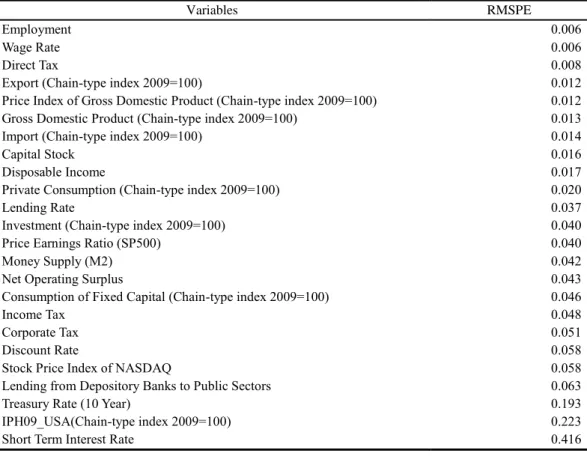
In total, the model for Japan consists of 33 simultaneous equations, comprising 24 estimated equations and 9 definitional identities, whilst the model for the United States consists of 35 simultaneous equations, comprising 23 estimated equations and 12 definitional identities. We conducted the final test from the first quarter 2009 to the third quarter 2016 (Quarterly). Table 6 and
Table 7 show the root mean square percentage error (RMSPE)6 about selected variables of Japan and
the United States respectively. Some endogenous variables might not be satisfactory. However, the overall performance of this system is acceptable.
5 GDP deflator in the USA is evaluated in 2009 Price
6 RMSPE shows the evaluation of model fitness. RMSPE = √ ∑ {( ̂ − )/ }
= where is
the actual observation time series, ̂ denotes the estimated time series, and represents the
17
Table 6. Evaluation of Model Performance of Japan by RMSPE
Variables RMSPE
Employment 0.002
Price Index of Gross Domestic Product (Chain-type index 2011=100) 0.005
Lending from Depository Banks to Public Sectors 0.006
Wage Rate 0.006
Consumption of Fixed Capital 0.008
Gross Domestic Product (Chain-type index 2011=100) 0.009
Private Consumption (Chain-type index 2011=100) 0.013
Disposable Income 0.013
Investment (Chain-type index 2011=100) 0.018
Import (Chain-type index 2011=100) 0.024
Corporate Tax 0.031
Income Tax 0.033
Direct Tax 0.035
Export (Chain-type index 2011=100) 0.039
Net Operating Surplus 0.050
Money Supply (M2) 0.052
Lending Rate 0.055
Discount Rate 0.057
Tokyo Stock Price Index 0.073
Loans from Central Bank to Depository Banks 0.098
Price Earnings Ratio 0.168
Interest Rate of Government Bond (10 Year) 0.556
Short Term Interest Rate 3.833
Table 7. Evaluation of Model Performance of the U.S. by RMSPE
Variables RMSPE
Employment 0.006
Wage Rate 0.006
Direct Tax 0.008
Export (Chain-type index 2009=100) 0.012
Price Index of Gross Domestic Product (Chain-type index 2009=100) 0.012
Gross Domestic Product (Chain-type index 2009=100) 0.013
Import (Chain-type index 2009=100) 0.014
Capital Stock 0.016
Disposable Income 0.017
Private Consumption (Chain-type index 2009=100) 0.020
Lending Rate 0.037
Investment (Chain-type index 2009=100) 0.040
Price Earnings Ratio (SP500) 0.040
Money Supply (M2) 0.042
Net Operating Surplus 0.043
Consumption of Fixed Capital (Chain-type index 2009=100) 0.046
Income Tax 0.048
Corporate Tax 0.051
Discount Rate 0.058
Stock Price Index of NASDAQ 0.058
Lending from Depository Banks to Public Sectors 0.063
Treasury Rate (10 Year) 0.193
IPH09_USA(Chain-type index 2009=100) 0.223
18
3.3.
Scenario Simulation
3.3.1. Baseline Simulation
We assume that this system in the post-sample period is from the fourth quarter 2016 to fourth quarter of 2050 (quarterly). In order to estimate the whole model in the post sample period, we are required to make the data for the exogenous variables in the post-sample in advance. Some variables are created along with their trends, whereas the others are set at a constant value at the end of sample the fourth quarter 2016. Especially, the policy interest rate is put in the third quarter of 2017 in order to avoid a discussion about exit strategy of monetary policy.
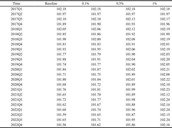
3.3.2. Scenario: Proposing A Possible Alternative Policy to the Current Monetary Stance
The central bank has relied heavily on unconventional monetary policy to tackle the deflation problem. Certainly, its unconventional monetary policy, including quantitative easing (QE) and credit easing (CE), might have expanded their capacity to influence monetary markets and financial conditions and the economy, compared to conventional monetary policy based on instrument of policy interest rate. However, they have not yet achieved the goal of overcoming deflation. For this reason, it is doubtful that current monetary policy has the power to overcome the deflation problem.
Deflation is thought to reflect weaknesses in the real economy. Thus, it would be required to examine an alternative solution using approaches based on the real economy. To do so, we conduct a scenario simulation to examine whether an improvement of wage rate would have an impact on prices. This simulation attempts to show an alternative solution to current monetary policy. Specifically, if wage rate is improved by 0.1 percent, 0.5 percent, and 1 percent toward baseline values, respectively, from the fourth quarter of 2016 to the fourth quarter of 2022, we examine how the GDP deflator would change.
3.3.3. Simulated Results
19
Table 8. Movement of GDP Deflator by Percent Change of Wage Rate of Japan
Time Baseline 0.1% 0.5% 1%
2017Q1 102.18 102.18 102.18 102.18
2017Q2 101.97 101.97 101.97 101.97
2017Q3 102.10 102.10 102.13 102.17
2017Q4 101.89 101.90 101.93 101.96
2018Q1 102.05 102.06 102.12 102.19
2018Q2 101.85 101.86 101.92 101.99
2018Q3 101.98 102.00 102.08 102.19
2018Q4 101.81 101.83 101.91 102.01
2019Q1 101.93 101.95 102.06 102.19
2019Q2 101.77 101.79 101.90 102.03
2019Q3 101.88 101.91 102.04 102.20
2019Q4 101.74 101.77 101.90 102.05
2020Q1 101.84 101.87 102.02 102.21
2020Q2 101.71 101.75 101.89 102.08
2020Q3 101.80 101.84 102.01 102.22
2020Q4 101.68 101.72 101.89 102.10
2021Q1 101.76 101.81 101.99 102.23
2021Q2 101.65 101.70 101.89 102.12
2021Q3 101.72 101.77 101.98 102.24
2021Q4 101.62 101.67 101.88 102.14
2022Q1 101.68 101.74 101.96 102.24
2022Q2 101.59 101.65 101.87 102.15
2022Q3 101.65 101.71 101.95 102.24
2022Q4 101.56 101.62 101.86 102.16
Table 9. Movement of GDP Deflator by Percent Change of Wage Rate of the U.S.
Time Baseline 0.1% 0.5% 1%
2017Q1 109.03 109.14 109.58 110.13
2017Q2 111.16 111.28 111.73 112.29
2017Q3 110.06 110.17 110.61 111.17
2017Q4 109.76 109.88 110.36 110.97
2018Q1 108.61 108.73 109.21 109.80
2018Q2 108.62 108.74 109.21 109.81
2018Q3 110.01 110.13 110.61 111.21
2018Q4 109.09 109.22 109.74 110.39
2019Q1 109.13 109.26 109.78 110.42
2019Q2 108.52 108.64 109.15 109.79
2019Q3 109.69 109.81 110.32 110.96
2019Q4 108.80 108.94 109.48 110.17
2020Q1 109.23 109.37 109.91 110.59
2020Q2 108.52 108.65 109.18 109.85
2020Q3 109.44 109.57 110.09 110.75
2020Q4 108.95 109.09 109.65 110.35
2021Q1 109.41 109.55 110.11 110.81
2021Q2 108.88 109.01 109.56 110.24
2021Q3 109.50 109.64 110.18 110.85
2021Q4 109.45 109.59 110.17 110.88
2022Q1 109.85 109.99 110.55 111.26
2022Q2 109.58 109.72 110.28 110.97
2022Q3 109.95 110.08 110.63 111.32
20
4.
Conclusion
This paper constructed a financial model, linked to a macroeconometric model, that reflects the central bank’s balance sheet to address how the monetary policy employed by central banks impacts the real economy through other depository banks. We then used the two linked models to examine improvement of wage rate and the impact on the movement of GDP price deflator. According to the results, when wage rates rise, it eventually leads to positive impact on GDP deflator through some markets. Hence, there might be a possibility that the rise of wage rate could become an alternative solution to current monetary policy, which aims to tackle the problem of deflation. We might be required to reconsider the current stance in that the economy is relying too heavily on current monetary policy based on QE and CE for overcoming the problem of deflation.
On the other hand, in the future, we should extend this model to improve its applicability to policy analysis. First, this study did not cover the implementation of optimal control, but we would be required to conduct simulations employing the optimal control of monetary policy, which could provide further insights about how best to conduct monetary policy. Second, optimal control of monetary policy should be simulated by linking Japan and the US. While scenario simulations were conducted for Japan and the US individually, we have not extended to simulating economic impacts by interrelation between two countries. Third, we should construct a model based on the balance sheet for government and link this to the financial model/macroeconometric model because it is indispensable to see the relation among monetary policy, fiscal policy, and real economy for better discussion about more appropriate remedies for deflation and the economy. Finally, the macroeconometric model should be modified into a more applicable framework for analyzing real economy sufficiently. Certainly, the performance and usability of the macroeconometric model based on Klein might be better than other types of macro models. However, it is so simple and intuitive that it could not determine the detailed causes of related issues. Indeed, to address the core of mechanisms of deflation, we would be required to have profound insights into not only wage rate but also labor productivity related to wage rate. To do so, the macroeconomic sector would be needed to be replaced by a multi-country/multi-sector econometric model which has a mechanism of microeconomic foundation.
21
References
Bernanke, B.S. and V. R. Reinhart. 2004. “Conducting Monetary Policy at Very Low Short-Term
Interest Rates.” American Economic Review, Vol. 9, No.4, pp. 27-48.
Bernanke, B.S., V. R. Reinhart., and B.P. Sack. 2004. “Monetary Policy Alternatives at the Zero
Bound: An Empirical Assessment.” Brooking Papers on Economic Activity, Vol. 35, No.2, pp.
85-90.
Chow, G.C. 1975, Analysis and Control of Dynamic Economic Systems, New York: Wiley.
Cúrdia, V. and M. Woodford. 2011 “The Central-Bank Balance Sheet as an Instrument of Monetary
Policy.” Journal of Monetary Economics, Vol. 58, No.1, pp. 54-79.
Eggertsson, G.B., and N. R. Mehrotra. 2014. “A Model of Secular Stagnation.” NBER Working Paper
20574.
Friedlaender, A. F. 1973. “Macro Policy Goals in the Postwar Period:A Study in Revealed Preferences,”
The Quarterly Journal of Economics, Vol. 87(2), pp. 25–43.
Honda, Y. 2014. “The Effectiveness of Nontraditional Monetary Policy: The Case of Japan.” The
Japanese Economic Review, Vol. 65, No. 1, March 2014.
Kuroda, H. 2016. “The Battle Against Deflation: The Evolution of Monetary Policy and Japan’s
Experience (Speech at Columbia University in New York).” The Bank of Japan.
Klein, L.R. 1964. “The Keynesian Revolution Revisited.” Economic Studies Quarterly, Vol. XV, No.
1, pp. 1-24.
Klein, L.R. 1983. Lectures in Econometrics, Amsterdam: North-Holland.
Klein,L.R. and W.Krelle,1983,Capital Flows and Exchange Rate Determination, Journal of Economics, Supplement 3.
Kosaka, H. 2017. “The Monetary Modeling for Conventional and Unconventional Monetary Policy.”
SFC Discussion Paper, SFC-DP, 2016-006. (in Japanese)
Miyao, R. 2006. Time series analysis of macroeconomic monetary policy. Tokyo: Nihon Keizai
Shinbunsha. (in Japanese)
Nelson, C.H. and A.F. Siegel. 1987. “Parsimonious Modeling of Yield Curves.” Journal of Business,
Vol. 60, No. 4, pp. 473-489.
Pissarides, C.A. 1972. “A Model of British Macreconomic Polict, 1955-1969.” Manchester School of
Economic and Social Studies, Vol. 40, pp.245-259.
22
Appendix A. Framework of Macroeconometric Model
This section illustrates the macroeconometric model. We follow Klein’s skeleton model (1983). We partially extend this conventional model for making the transmission channel of monetary policy to
macro economy7.
Endogenous Variables
: Gross domestic product (real) : Employment : Private final consumption (real) : Labor force : Gross fixed capital formation (real) � : Wage rate
: Exports (real) : Interest rate (real)
: Imports (real) , : Indirect tax (nominal)
: Capital stock (real) , : Direct tax (nominal)
: Depreciation (real) , : Corporation profit tax (nominal)
: National income (nominal) , : Transfer payments (nominal)
� : Corporation profit (nominal) : Exchange rate : GDP deflator
Exogenous Variables
: Government final consumption (real) : Population : World trade transactions (real) �, : World trade price
: Money supply (nominal) , : Import price
Identities
Real GDP
= + + + − (A.1)
Nominal GDP
= + ( , + , + , − , ) − (A.2)
National income
� + � = + ( , + , − , ) (A.3)
23
Capital stock
= − + − (A.4)
Behavior and Technological Relations
Consumption
= + ( ) + ( −
− ) + � , (A.5)
Investment
= + + + − + � , (A.6)
Export
= + + ( �,) + − + � , (A.7)
Import
= + +
, + − + � ,
(A.8)
Employment
log = + log + log − + − + � , (A.9)
Price formation
= + (� ) + , + � , (A.10)
Wage fate
� = ℎ + ℎ ( ) + ℎ + � , (A.11)
Labor force
24
Velocity of circulation of money
log ( ) = + + Δ log + � ,
< , >
(A.13)
Depreciation
= + − + � , (A.14)
Indirect tax
, = + + � , (A.15)
Indirect tax
, = + + � , (A.16)
Corporation tax
, = + � + � , (A.17)
Transfer payments
, = + − + � + � , (A.18)
Exchange Rate
log = + log + − − ( − ) + � ,
> , > , >
25
Appendix C. Estimated Results
This section will show the estimated results. All equations are basically by ordinary leas squares. The t-statistic is shows in parentheses, and the p-values is represented in brackets.
B.1 Japan
Macroeconomic Sector
(B.1) Consumption (Real)
CP11_JPN/POP_JPN=35.6820373138 (6.238)
[0.000]
+6.94917525766*LOG(YD_JPN/(POP_JPN*PGDP11_JPN)) (3.690)
[0.001]
+0.226319255741*CP11_JPN(-4)/POP_JPN(-4) (1.881)
[0.065]
+[AR(1)=0.892588205564,UNCOND,ESTSMPL="2000Q1 2016Q4"] (13.629)
[0.000]
Adj.R =0.945 S.E.=0.203 D.W.=2.394
(B.2) Investment (Real)
LOG(I11_JPN)=4.42092823551 (1.607) [0.113]
+0.53668968935*LOG(GDP11_JPN(-2)) -0.000832360776107*R_GB_JPN(-4) (2.559) (-0.048)
[0.013] [0.962]
+[AR(1)=0.955588712446,UNCOND,ESTSMPL="2001Q1 2017Q3"]
(23.517) [0.000]
Adj.R =0.928 S.E.=0.020 D.W.=1.368
(B.3) Export (Real)
26
(86.079) (11.856) [0.000] [0.000]
+0.589450548819*LOG(PWT10_SA(-2)/PGDP11_JPN(-2)) (4.786)
[0.000]
-0.147132137808*DM08Q4_09Q1 (-2.368)
[0.021]
+[AR(1)=0.970955815439,UNCOND,ESTSMPL="2000Q1 2017Q1"] (17.769)
[0.000]
Adj.R =0.969 S.E.=0.039 D.W.=2.117
(B.4) Import (Real)
IM11_JPN=-1344096.87692 (-6.707) [0.000]
+104625.513862*LOG(GDP11_JPN) +0.635523348833*IM11_JPN(-1) (6.724) (11.490)
[0.000] [0.000]
Adj.R =0.963 S.E.=1762.95 D.W.=1.619
(B.5) Disposable Income
LOG(YD_JPN)=-8.217248294 (-4.361) [0.000]
+1.10772895271*LOG(PGDP11_JPN*GDP11_JPN (10.437)
[0.000]
-(TAX1_JPN_SA+TAX2_JPN+TAX3_JPN+TR_JPN)-DD_JPN) (2.884)
[0.005]
+[AR(1)=0.4219310745,UNCOND,ESTSMPL="2000Q1 2016Q4"] (5.359)
[0.000]
27 (B.6) Depreciation (Real)
LOG(DD_JPN/PGDP11_JPN)=0.336441467612*LOG(K05_JPN(-6)) (316.380)
[0.000]
+[AR(1)=0.956477591954,UNCOND,ESTSMPL="2000Q1 2016Q4"] (29.299)
[0.000]
Adj.R =0.968 S.E.=0.010 D.W.=2.191
(B.7) Labor Force
LOG(L_JPN_SA)=-0.155441063594+0.080285839178*LOG(GDP11_JPN) (-1.065) (4.667)
[0.291] [0.000]
-0.00526852217268*LOG(K05_JPN(-4))+0.908758034977*LOG(L_JPN_SA(-1)) (-0.430) (21.907)
[0.669] [0.000]
Adj.R =0.985 S.E.=0.003 D.W.=2.212
(B.8) Wage Rate
LOG(WAGE_RATE_JPN)=-0.746772694431 (-1.772)
[0.081]
+0.168529342246*LOG(GDP11_JPN(-1)/L_JPN_SA(-1)) (2.815)
[0.007]
+0.34780157233*LOG(PGDP11_JPN(-3)) (3.752)
[0.000]
+0.338824044813*LOG(WAGE_RATE_JPN(-4)) (3.061)
[0.003]
+[AR(1)=0.771077056717,UNCOND,ESTSMPL="2000Q1 2017Q1"]
(9.426) [0.000]
28 (B.9) Capital
K05_JPN =1.00354908898*(K05_JPN(-1) +I11_JPN+DD_JPN/PGDP11_JPN) (3461.525)
[0.000]
Adj.R =0.999 S.E.=2742196. D.W.=1.696
Monetary Sector
(B.10) Loans of Depository Banks from Central Bank
LC_JPN=1847.52982691+0.0614055916634*LB_JPN (0.004) (0.588)
[0.997] [0.559]
-127.016588859*(R_S_JPN(-2)-R_D_JPN(-2))/R_S_JPN(-1) (-0.104)
[0.917]
-1830.13393059*(R_DT_JPN(-2))/R_S_JPN(-1)-199947.472083*DM00Q1_17Q4 (-0.245) (-5.556)
[0.807] [0.000]
+ [AR(1)=0.911391242,UNCOND,ESTSMPL="2000Q3 2016Q4"] (17.605)
[0.000]
Adj.R =0.964 S.E.=30081.96 D.W.=2.465
(B.11) Lending of Depository Banks to Private sectors
LOG(LB_JPN)=13.5676608094 (16.673)
[0.000]
+0.0884609014423*LOG(IPF11_JPN(-4)+IPH11_JPN(-4)) (1.135)
[0.262]
+0.0512102295042*LOG(LC_JPN(-2)+CT1_JPN(-2)+CT2_JPN(-2)+CT3_JPN(-2)) (2.272)
[0.027]
-0.0289762107245*R_S_JPN/R_L_JPN(-1) +0.0170718979549*DM08Q4_09Q1 (-0.839) (4.758)
[0.405] [0.000]
29
(36.465) [0.000]
Adj.R =0.978 S.E.=0.008 D.W.=1.445
(B.12) Money Supply
LOG(M2_JPN)=5.53246598416+0.170572884313*LOG(MRS_JPN(-4)) (2.462) (9.932)
[0.017] [0.000]
+0.513652899842*LOG(LB_JPN) (3.254)
[0.002]
Adj.R =0.823 S.E.=0.048 D.W.=0.637
(B.13) Short-term Interest Rate
R_S_JPN=-0.0118140365167+0.0954354190102*R_M_JPN(-1)+2.52732417778*R_DT_JPN (-1.070) (1.945) (21.268)
[0.289] [0.056] [0.000] +[AR(1)=0.50422743373,UNCOND,ESTSMPL="2000Q2 2017Q1"]
Adj.R =0.968 S.E.=0.030 D.W.=1.696
(B.14) Discount Rate
R_D_JPN=0.269789497607+0.95500048406*R_M_JPN (4.799) (22.067)
[0.000] [0.000]
+[AR(1)=0.940452257824,UNCOND,ESTSMPL="2000Q1 2017Q1"] (23.536)
[0.000]
Adj.R =0.952 S.E.=0.041 D.W.=2.010
(B.15) Lending Rate
R_L_JPN=1.09339182261+0.170336898266*R_GB_JPN(-1) (4.428) (3.462)
[0.000] [0.001]
+[AR(1)=0.982269034473,UNCOND,ESTSMPL="2000Q2 2017Q1"]
30 (B.16) Long-term Interest Rate
R_GB_JPN=3.70975352645-3.66783490686e-05*M2_JPN/PGDP11_JPN
(4.540) (-3.294)
[0.000] [0.002]
+0.563734694541*R_S_JPN+0.402083900874*@PCH(INDEX_TOPIX) (1.308) (1.902)
[0.196] [0.062]
+[AR(1)=0.853641644347,UNCOND,ESTSMPL="2000Q2 2017Q1"] (14.727)
[0.000]
Adj.R =0.922 S.E.=0.144 D.W.=1.531
(B.17) Price-to-Earnings Ratio (P/E Ratio)
LOG(PER_NON_JPN)=3.83037598027+1.68022680997*DLOG(GDP11_JPN(-4)) (4.191) (0.656)
[0.000] [0.514]
+0.0495479127532*LOG(PER_NON_JPN(-4)) (0.650)
[0.519]
+[AR(1)=0.948289886032,UNCOND,ESTSMPL="2001Q2 2017Q1"] (22.050)
[0.000]
31
B.2 The United States
Macroeconomic Sector
(B.18) Consumption (Real)
CP09_USA/POP_USA=0.00128840769754 (-3.806)
[0.000]
+0.547571008698*YD_USA/(POP_USA*(PGDP09_USA/100)) (8.223)
[0.000]
+0.444656906691*CP09_USA(-4)/POP_USA(-4) (6.612)
[0.000]
Adj.R =0.993 S.E.=0.000 D.W.=0.281
(B.19) Investment (Real)
LOG(I09_USA)=1.27559733638+0.0232830595194*LOG(GDP09_USA(-2)) (1.397) (0.173)
[1.656] [0.863]
-0.0221570402876*R_GB_USA(-4)+0.822940559904*LOG(I09_USA(-4)) (-2.982) (13.266)
[0.004] [0.000] -0.140569183581*DM08Q4_10Q4
(-8.138) [0.000]
Adj.R =0.972 S.E.=0.047 D.W.=0.307
(B.20) Export (Real)
EX09_USA=-2049.66642479+160.770226895*LOG(WT_SA)
(-7.002) (7.187)
[0.000] [0.000]
+71.9717320025*LOG(PWT10_SA(-4)/PGDP09_USA(-4)) (1.784)
[0.078]
+0.807030884462*EX09_USA(-2)-202.171766121*(DM09Q1+DM09Q2) (29.300) (-7.625)
32
Adj.R =0.992 S.E.=35.725 D.W.=0.924
(B.21) Import (Real)
IM09_USA=-703.960300382+0.124844256416*GDP09_USA
(-7.529) (9.126)
[0.000] [0.000]
+207.912382243*LOG(PGDP09_USA(-4)/PIM09_USA(-4)) (3.775)
[0.000]
+0.505548499992*IM09_USA(-2)-253.169776275*(DM09Q1+DM09Q2) (9.963) (-9.505)
[0.000] [0.000]
Adj.R =0.998 S.E.=35.186 D.W.=0.626
(B.22) Disposable Income
YD_USA=-219.074012981 (-5.879) [0.000]
+0.965015929011*((PGDP09_USA/100)*GDP09_USA- (TAX1_USA+TAX2_USA+TAX3_USA-TR_USA)-DD09_USA*(PGDP09_USA/100))
(258.115) [0.000]
Adj.R =0.998 S.E.=126.435 D.W.=0.638
(B.23) Depreciation (Real)
DD09_USA=0.156775811286*KK09_USA(-4)-248.434921183*DM08Q1_09Q2 (155.699) (-5.946)
[0.000] [0.000]
-40.296036036*@SEAS(1)+22.1961379053*@SEAS(4) (-1.818) (0.994)
[0.072] [0.322]
Adj.R =0.965 S.E.=97.422 D.W.=9.235
(B.24) Labor Force
33
(2.802) [0.006]
-0.0318535373752*LOG(KK09_USA(-4))+0.924113586204*LOG(L_USA(-1)) (-6.607) (39.366)
[0.000] [0.000]
-0.0157358777426*DM09Q1+0.00265931128749*@SEAS(1) (-4.611) (3.695)
[0.000] [0.000]
Adj.R =0.998 S.E.=0.003 D.W.=1.319
(B.25) Wage Rate
LOG(WAGE_RATE_USA)=-1.98475633034+1.44289323265*LOG(GDP09_USA(-4)/L_USA(-4)) (-4.428) (19.271)
[0.000] [0.000]
+0.518412360733*LOG(PGDP09_USA) (8.550)
[0.000]
Adj.R =0.997 S.E.=0.015 D.W.=0.467
(B.26) Capital
KK_USA/PGDP09_USA-(KK_USA(-4)/PGDP09_USA(-4))=1.25848852041 (1.302)
[0.198]
+0.013653978003*(I09_USA-DD09_USA) (4.739)
[0.000]
+[AR(1)=0.752431375737,UNCOND,ESTSMPL="2000Q1 2016Q4"] (7.797)
[0.000]
Adj.R =0.867 S.E.=1.896 D.W.=2.060
Monetary Sector
(B.27) Lending of Depository Banks to Private sectors
34
[0.000] [0.000]
+965739.874897*LOG(A_LN+A_CG) (6.353)
[0.000]
-1796526.30401*R_S_USA/R_L_USA(-1) (-3.184)
[0.002]
Adj.R =0.855 S.E.=523884.1 D.W.=0.121
(B.28) Money Supply
M2_USA_SA=1646.58343762+0.000988630963668*MRS_USA+0.000791109223839*LB_USA
(6.432) (20.330) (16.144)
[0.000] [0.000] [0.000]
Adj.R =0.986 S.E.=283.165 D.W.=0.221
(B.29) Short-term Interest Rate
R_S_USA=-0.0235230475373+0.963819647635*R_M_USA+0.149001827503*R_DC_USA(-2) (-1.287) (21.598) (2.219)
[0.208] [0.000] [0.034]
Adj.R =0.967 S.E.=0.047 D.W.=1.032
(B.30) Discount Rate
R_D_USA =0.650395000814+1.05545019766*R_M_USA-0.31926703244*DM09Q1_Q4 (16.657) (61.656) (-2.729)
[0.000] [0.000] [0.000]
Adj.R =0.986 S.E.=0.222 D.W.=0.208
(B.31) Lending Rate
R_L_USA=3.38571104083+0.301746187763*R_GB_USA (2.093) (2.575)
[0.041] [0.013]
+[AR(1)=0.961590044375,UNCOND,ESTSMPL="2003Q1 2017Q3"] (27.967)
[0.000]
35 (B.32) Long-term Interest Rate
R_GB_USA=5.5267305013-0.0488501996479*M2_USA_SA/PGDP09_USA (9.385) (-8.386)
[0.000] [0.000]
+0.143339137758*R_S_USA(-2)+0.0762762828759*PER_SP500 (2.446) (3.628)
[0.018] [0.001]
+[MA(1)=0.727992795853,UNCOND,ESTSMPL="2003Q1 2017Q3"] (6.045)
[0.000]
Adj.R =0.926 S.E.=0.284 D.W.=1.669
(B.33) Price-to-Earnings Ratio (P/E Ratio)
PER_SP500=-2.37245419837+0.00026764986143*GDP09_USA (-0.936) (1.892)
[0.353] [0.063]
+0.932352666059*PER_SP500(-1) (29.228)
[0.000]
36
Appendix C. Balance Sheet
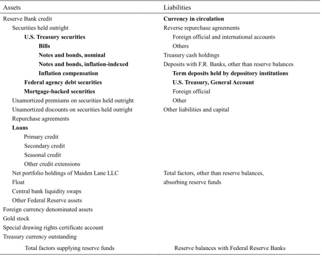
Table 10 and Table 11 represent the balance sheet of the Bank of Japan and the Federal Reserve. The items which are employed as endogenous variables into the financial model are in bold texts. The relations of identities based on balance sheets is explained in Kosaka (2016)
.
Table 10.Balance Sheet of Bank of Japan
Assets Liabilities
Claims on Nonresidents
Claims on Government Claims on Depository
Claims on Other Financial Corporations Claims on Other Sectors
Monetary Base
Cash Currency Issued Current Account Balances
Labilities to Nonresidents
Liabilities to Government
Other Items (Net)
Table 11.Balance Sheet of the Federal Reserve
Assets Liabilities
Reserve Bank credit Securities held outright U.S. Treasury securities Bills
Notes and bonds, nominal Notes and bonds, inflation-indexed Inflation compensation
Federal agency debt securities Mortgage-backed securities
Unamortized premiums on securities held outright Unamortized discounts on securities held outright Repurchase agreements
Loans
Primary credit Secondary credit Seasonal credit Other credit extensions
Net portfolio holdings of Maiden Lane LLC Float
Central bank liquidity swaps Other Federal Reserve assets Foreign currency denominated assets Gold stock
Special drawing rights certificate account Treasury currency outstanding
Currency in circulation
Reverse repurchase agreements
Foreign official and international accounts Others
Treasury cash holdings
Deposits with F.R. Banks, other than reserve balances
Term deposits held by depository institutions U.S. Treasury, General Account
Foreign official Other
Other liabilities and capital
Total factors, other than reserve balances, absorbing reserve funds