胡 波 Hu Bo

 

早稲田大学大学院 環境・エネルギー研究科

博士学位論文

 

   

A New Hierarchical Fault Diagnosis Method for  Power Distribution Networks with PV Systems 

‐‐‐Equivalent‐Input‐Disturbance‐Based Approach‐‐‐ 

 

太陽光発電システムを含む配電ネットワーク に関する新しい階層的故障診断手法

― 等価入力外乱手法によるアプローチ ―

 

 

 

   

2013

年

  02

月

 

   

胡 波

Hu  Bo 

ABSTRACT 

Modern  power  system  is  huge  and  complex.  State  monitoring  and  fault  diagnosis  are  necessary  to  guarantee  its  stability  and  safety.  The  traditional  fault  diagnosis  methods  for  distribution network are mainly based on a large amount of sensor information and a complete  model  of  distribution  network.  These  methods  have  solved  the  fault  diagnosis  problems  in  a  certain  degree,  but  still  remains  some  shortcomings,  such  as  high  dependency  of  sensor  information  and  enormous  size  of  fault  diagnosis  model.  Moreover,  with  the  penetration  of  grid‐connected PV generation, the conventional fault diagnosis method encounter an increasing  number of bottlenecks, such as fluctuation of PV output and malfunctions of protective relays  caused by PV power injection. 

The doctoral dissertation concerns the above problems and presents a new hierarchical fault  diagnosis (HFD) method for power distribution network that is based on a hierarchical model  and the equivalent‐input‐disturbance (EID) approach. 

Due  to  the  complexity  of  power  distribution,  a  complete  model  of  an  entire  distribution  is  extremely  complicated.  Therefore,  a  hierarchical  technology  is  applied  to  build  a  hierarchical  model  of  distribution  network  for  fault  diagnosis.  Fault  diagnosis  is  carried  out  from  the  top  down through the layers to gradually locate a fault and to identify its type. 

While faults occur, the faults will cause large disturbances to the system from the standpoint  of power supply. Based on this concept, the EID approach, which can estimate the magnitude of  system disturbances, is used to diagnose the faults. To eliminate the influence of PV for the fault  diagnosis, the fault signal is abstracted by removing the PV output fluctuation from EID. 

Unlike  conventional  methods,  the  proposed  method  uses  the  hierarchical  model  for  fault  diagnosis, which reduces the complexity involved in modeling, shortens the computation time  and  does  not  need  a  large  amount  of  sensor  information.  Furthermore,  our  fault  diagnosis  method shows a good performance in the case of PV generation embedded in the feeder. The  simulations on IEEE 37 nodes radial distribution test feeder model demonstrate the validity and  superiority of the HFD method. 

 

ii 

ACKNOWLEDGMENTS 

I  would  like  to  express  my  acknowledgements  to  all  the  persons  who  helped  me  during  the  writing of this thesis. 

My deepest gratitude goes first and foremost to my supervisor, Professor R. Yokoyama, for his  support, patience, and consistent encouragement throughout the course of my Ph.D study. His  technical advice was essential to the successful completion of this dissertation. I also would like  to acknowledge my co‐advisor Professor J. She of Tokyo University of Technology. During my  three‐year  doctoral  study,  he  provided  me  many  invaluable  guidance  for  my  research  and  helped me to revise the papers strictly. 

Moreover, I want to thank the other members of my review committees, Professor M. Katsuta,  and Professor S. Tomonari for their helpful comments during the grueling thesis review process. 

I  am  also  grateful  to  Dr.  Y.  Zhou  of  the  Fujitsu  Limited  Company,  Professor  M.  Wu  of  Central  South University. They provided me with selfless help and guidance whatever in my study or in  my life. 

To  my  family  and  friends,  I  dedicate  my  heartfelt  thanks  and  gratitude  for  the  support  and  encouragement that they provided me through my entire life. None of my achievements would  have been possible achieved without them in these years. 

In  addition,  it  is  also  a  pleasure  to  thank  my  colleagues  from  Yokoyama  laboratory  for  their  support  and  help.  I  must  acknowledge  Dr.  H.  Magori,  Dr.  T.  Nimura  and  Dr.  K.  Koyanagi  for  teaching  me  many  basic  skills  and  background  knowledge  on  power  system.  I  also  give  my  thanks  to  the  doctoral  students  D.  Yamasida,  Y.  Hida,  J.  Zhang,  and  M.  Ding  for  all  of  their  computer and technical  assistance in  my study, and special thanks to  our administrative staff  Mrs Y. Inaba and Mrs H. Kano for their guidance of the doctoral review procedures. 

Financial support from the “National Construction High level University Government‐sponsored  Graduate  Student  Project”  provided  by  the  China  Scholarship  Council  is  also  gratefully  acknowledged. 

Bo  Hu    Jan.  2013 

Contents 

ABSTRACT  i

ACKNOWLEDGMENTS  ii

Contents  i

List of Figures  iii

List of Tables  vi

Abbreviations  vii

   

Chapter 1  1

Background and Research Outline  1

1.1 Chapter Introduction  1

1.2 Faults in Electrical Power System  2

1.2.1 Electrical Power System  2

1.2.2 Faults Definition and Classification  2

1.2.3 Fault Types in the Three‐Phase Network  3

1.3 Conventional Fault Diagnosis Methods  4

1.3.1 Monitoring Information‐Based Approach  6

1.3.2 Model‐Based Fault Diagnosis Approach  7

1.4 Influence of PV Installation  8

1.5 Research Outline  9

Chapter References  12

   

Chapter 2  15

Hierarchical Fault Diagnosis Model of Power Distribution Networks  15

2.1 Chapter Introduction  15

2.2 HFD Model Construction  16

2.2.1 Framework of HFD Model  16

2.2.2 Procedures of HFD Algorithm  19

2.3 Model Parameters Calculation Algorithm  20

2.3.1 Basis of BFS Algorithm  20

2.3.2 Improved BFS Algorithm  22

2.4 Dynamic Model for Load Cluster  28

2.5 Application to IEEE‐13 Feeder Model  30

2.5.1 Data of IEEE‐13 Feeder Model  30

2.5.2 Hierarchical Framework of IEEE‐13 Feeder  32

2.5.3 Model Parameters Calculation Results  34

2.5.4 Dynamic of Load Clusters  39

2.6 Conclusion  42

Chapter References  43

   

Chapter 3  44

Fault Diagnosis Method of Power Distribution Networks Based on EID Approach  44

3.1 Chapter Introduction  44

3.2 Concept of EID Approach  45

3.2.1 Definition of EID  45

3.2.2 Estimation of EID  47

3.2.3 Design of Filter and State Observer  49

3.3 Key Technologies of Fault Diagnosis  51

ii 

3.3.1 Fault Disturbance  51

3.3.2 Thresholds of EIDs  55

3.3.3 Characteristics of Faults  56

3.4 Application to a Load Cluster  57

3.5 Conclusion  61

Chapter References  62

   

Chapter 4  64

Fault Diagnosis of Distribution Networks with PV Generation Embedded  64

4.1 Chapter Introduction  64

4.2 Impacts of Grid‐connected PV Generation  65

4.2.1 Grid‐connected PV Generation  65

4.2.2 Reverse Power  69

4.2.3 Electrical line losses  72

4.2.4 Protection System Malfunction  73

4.3 Dynamic Model of Distribution Network with PV Generation  76

4.4 Eliminate the Impacts of PV Generation  78

4.4.1 Impacts of PV Disturbances on Fault Diagnosis  78

4.4.2 Calculate the EID of PV Disturbances  80

4.4.3 Thresholds of EID  81

4.5 Application to a Test Model  81

4.5.1 Data of Test Model  81

4.5.2 Thresholds Setting  82

4.5.3 Components and Structure of Simulations  82

4.5.4 Simulation Results  84

4.6 Conclusion  87

Chapter References  89

   

Chapter 5  90

EID‐based HFD Method Applied to the IEEE 37 Nodes Test Feeder  90

5.1 Chapter Introduction  90

5.2 Data of IEEE‐37 Feeder  90

5.3 HFD Method for IEEE‐37 Feeder  94

5.3.1 HFD Model  94

5.3.2 Procedures of HFD Algorithm  99

5.4 Application to IEEE‐37 Feeder Model  99

5.4.1 Design of Fault Disturbances  99

5.4.2 Thresholds Setting for All Load Clusters  100

5.4.3 Simulation Results Analysis  101

5.5 Conclusion  107

Chapter References  108

   

Chapter 6  109

Conclusions and Further Works  109

6.1 Conclusion  109

6.2 Further Works  112

Chapter References  113

List of Publications  114

List of Figures 

Fig. 1‐1: Block diagram of an electrical power system.  2 

Fig. 1‐2: Type of faults on a Three Phase System.  4 

Fig. 1‐3: Configuration of a fault diagnosis system with function distributed.  5 

Fig. 1‐4: Power flow of network.  9 

Fig. 2‐1: Schematic Diagram of Tokyo 23 districts distribution networks.  16  Fig. 2‐2: hierarchical framework of Tokyo 23 districts distribution networks.  17 

Fig. 2‐3: A three‐phase line section.  21 

Fig. 2‐4: Branch numbering scheme for radial distribution network.    21 

Fig. 2‐5: The flow chart of BFS algorithm.  23 

Fig. 2‐6: Flow chart of the BFS algorithm with PV­specified node compensation.  27 

Fig. 2‐7: Equivalent impedance of load cluster.  29 

Fig. 2‐8: Equivalent circuit of Cluster  C₁⁽¹⁾  in Layer 1.  29  Fig. 2‐9: IEEE 13 nodes radial distribution feeder (IEEE‐13 feeder).  31 

Fig. 2‐10: Tree structure of Fig. 2‐9.  32 

Fig. 2‐11: Hierarchical structure of IEEE‐13 feeder.  34 

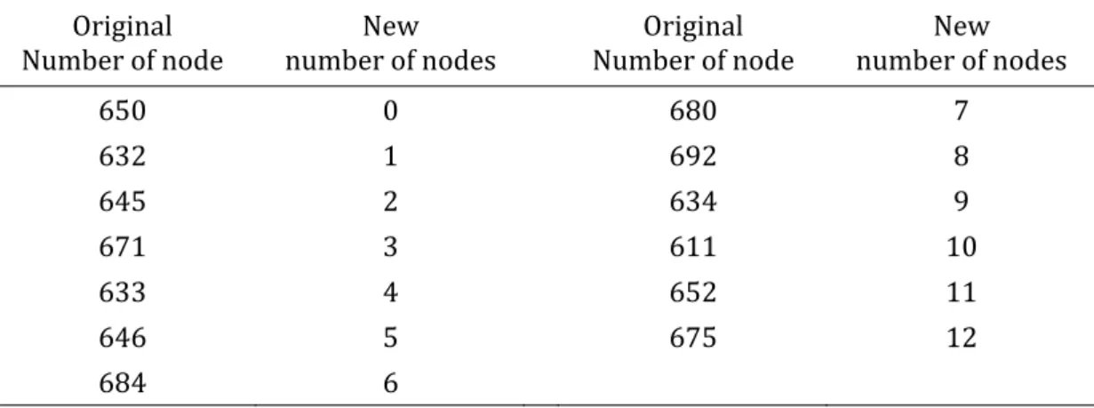
Fig. 2‐12: Nodal voltages of IEEE‐13 feeder without PV embedded.  35 

Fig. 2‐13: IEEE‐13 feeder with PV installation.  36 

Fig. 2‐14: Nodal voltages of IEEE‐13 feeder with PVs, which are PQ­specified nodes.  36  Fig. 2‐15: Nodal voltages of IEEE‐13 feeder with PVs, which are PV­specified nodes.  38 

Fig. 3‐1: Plant.  45 

Fig. 3‐2: Plant with EID.  46 

Fig. 3‐3: Configuration of disturbance estimation.  48 

Fig. 3‐4: (a) Three‐phase short circuit; (b) Simulation structure for short‐circuit fault.  52 

Fig. 3‐5: Three‐phase short circuit fault current.  53 

Fig. 3‐6: Simulation structure for EID approach.  54 

Fig. 3‐7: The EID of system in different situations.  54 

iv 

Fig. 3‐8: Load variation of a node during a 24‐hour period.  55 

Fig. 3‐9: Estimated state error,  Δi₁⁽¹⁾( )t .  57 

Fig. 3‐10: Normal load variation.  58 

Fig. 3‐11: Thresholds of EID.  58 

Fig. 3‐12: Faults: (a) amplitude type and (b) phase type.  59 

Fig. 3‐13: EID estimate,  dˆ ( )₁⁽¹⁾_e t   and  d&ˆ ( )₁⁽¹⁾_e t   of Cluster  C₁⁽¹⁾  in layer 1.  59 

Fig. 3‐14: Amplitudes and phases of  Iˆ₁⁽¹⁾.  60 

Fig. 4‐1: Block diagram of a PV grid‐connected system.  65 

Fig. 4‐2: PV output model.  68 

Fig. 4‐3: Load model.  68 

Fig. 4‐4: Load with PV penetration in spring model.  69 

Fig. 4‐5: Load with PV penetration in winter model.  69 

Fig. 4‐6: Sending voltage curve in spring model.  70 

Fig. 4‐7: Terminal voltage curve in spring model.  70 

Fig. 4‐8: Tap position.  70 

Fig. 4‐9: Sending voltage curve in winter model.  71 

Fig. 4‐10: Terminal voltage curve in winter model.  72 

Fig. 4‐11: Tap position.  72 

Fig. 4‐12: Electrical line losses of distribution feeder.  73 

Fig. 4‐13: Short circuit at position a.  74 

Fig. 4‐14: Simulation structure of short circuit fault with PV generation embedded.  75 

Fig 4‐15: The fault current of Relay R.  76 

Fig. 4‐16: Block diagram of distribution feeder with PV generation connected.  76 

Fig. 4‐17: Equivalent circuit of Fig. 4.16.  77 

Fig. 4‐18: EID estimates of system,  d tˆ ( )_e ,  d tˆ ( )&_e .  83  Fig. 4‐19: Simulation structure of fault diagnosis method based on EID approach.  83  Fig 4‐20: Load parameter variations when the short circuit fault occurs.  84 

Fig. 4‐21: EID estimates of system,  d tˆ ( )_e ,  d tˆ ( )&_e , while the PV output is stable.  84  Fig. 4‐22: EID estimates of PV generation,  dˆ ( )_pv t , while the PV output is stable.  85  Fig. 4‐23: PV variation, current ipv and resistance rpv.  85  Fig. 4‐24: EIDs estimates of system,  d tˆ ( )_e ,  d tˆ ( )&_e , while the PV output is variable.  86  Fig. 4‐25: EIDs estimates of PV  dˆ_{e_pv}( )t ,  dˆ&_{e_pv}( )t , while the PV output is variable.  86  Fig. 4‐26: EIDs estimates of load node,  dˆ ( )_{e_L} t ,  dˆ ( )&_{e_L} t , while the PV output is variable.  87  Fig. 4‐27: Errors of EID estimates between de(t) of scenario 1) and de_L(t) of the scenario 2).  87 

Fig. 5‐1: IEEE 37 nodes test feeder (IEEE‐37 feeder).  91 

Fig. 5‐2: Hierarchical structure of IEEE 37 nodes test feeder (IEEE‐37 feeder).  96  Fig. 5‐3: Faults in IEEE‐37 feeder: (a) amplitude type and (b) phase type.  100 

Fig. 5‐4: EID estimate,  dˆ ( )₂⁽²⁾_e t , for Layer 1.  101 

Fig. 5‐5: EID estimates,  dˆ₂⁽²⁾_−je( )t   and  d&ˆ₂⁽²⁾_−je( ) (t j=1,2,3,4), in Layer 2.  101  Fig. 5‐6: EID estimates,  dˆ_{2 3}⁽³⁾_{− −je}( )t   and  d&ˆ_{2 3}⁽³⁾_{− −je}( ) (t j=1,2,3), in Layer 3.  102  Fig. 5‐7: EID estimates,  dˆ_{2 4}⁽³⁾_{− −je}( )t   and  d&ˆ_{2 4}⁽³⁾_{− −je}( ) (t j=1,2,3,4), in Layer 3.  102  Fig. 5‐8: EID estimates,  dˆ_{2 3 3}⁽⁴⁾_{− − −je}( )t   and  d&ˆ_{2 3 3}⁽⁴⁾_{− − −je}( ) (t j=1, 2,3), in Layer 4.  103  Fig. 5‐9: EID estimates,  dˆ_{2 4 3}⁽⁴⁾_{− − −je}( )t   and  d&ˆ_{2 4 3}⁽⁴⁾_{− − −je}( ) (t j=1,2), in Layer 4.  103  Fig. 5‐10: EID estimates,  dˆ₂₃₃₃₂⁽⁵⁾ _e( )t and  d&ˆ₂₃₃₃₂⁽⁵⁾ _e( ) (t j=1,2,3), in Layer 5.  104  Fig. 5‐11: Amplitudes and phases of (a)  Iˆ_{2 3 4 2}⁽⁴⁾_{− − −}   (Node 718) and (b)  Iˆ_{2 3 2 2 2}⁽⁴⁾_{− − − −} (Node 732).  105   

vi 

List of Tables 

Table 2‐1: Transformer data of IEEE‐13 feeder  31 

Table 2‐2: Lengths of lines for IEEE‐13 feeder  31 

Table 2‐3: Nodal Active and reactive power of IEEE‐13 feeder  32 

Table 2‐4: Hierarchical structure of IEEE‐13 feeder  33 

Table 2‐5: New number of node  35 

Table 2‐6: Data of PV generations which are regarded as PQ‐specified node  36  Table 2‐7: Data of PV generations which are regarded as PV­specified node  37 

Table 2‐8: Reactive power of PV generation  39 

Table 2‐9: Dynamic model of load clusters without PV generations embedded  40  Table 2‐10: Dynamic model of load clusters with PV generations embedded, which are regarded 

as PQ‐specified node  41 

Table 2‐11: Dynamic model of load clusters with PV generations embedded, which are regarded 

as PV‐specified node  42 

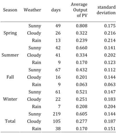
Table 4‐1: Data of PV during one year period  67 

Table 4‐2: Parameters of test system  82 

Table 5‐1: Transformer data of IEEE‐37 feeder  91 

Table 5‐2: Line section data of IEEE‐37 feeder  91 

Table 5‐3: Overhead line configurations of IEEE‐37 feeder  92 

Table 5‐4: Bus load data of IEEE‐37 feeder  93 

Table 5‐5: Data of PV generation  93 

Table 5‐6: Hierarchical structure of IEEE‐37 feeder  94 

Table 5‐7: Dynamic Model of Load Clusters for IEEE‐37 Feeder  97  Table 5‐8: Infinity and Euclidean norms of estimated EIDs of faulty load clusters  105  Table 5‐9: Infinity and Euclidean norms of estimated EIDs of normal load clusters  106 

 

Abbreviations 

 

HFD: hierarchical fault diagnosis  EID: equivalent‐input‐disturbance  PV: photovoltaic 

EMS: energy management system 

SCDA: supervisory control and data acquisition  BFS: backward and forward sweep 

LC: load cluster 

SISO: single‐input single‐output  MPPT: maximum power point tracking  PWM: pulse‐width modulation 

SNR: signal‐noise ratio 

PVNSM: PV­specified node sensitivity matrix   

Chapter 1 

Background and Research Outline 

1.1 Chapter Introduction 

The electrical power system represents not only one of the most complex artificial systems  in the world, but also one of the most significant ones in modern society. Power system are key  elements  of  modern  society,  providing  clean  and  convenient  energy  to  drive  motors,  light  houses and streets, run manufacturing plants and business, and power our communications and  computer systems. With the development of human society, the demand of electrical power is  ever‐increasing. In a word, the power system is the basic of modern human life, which plays a  vital and important role in maintaining the society operation. 

The stable and security operation is the most important issue for power system. When the  fault occurs, location and type of the fault should be identified exactly and rapidly to lessen the  loss  or  influence  of  fault.  The  traditional  fault  diagnosis  methods  for  power  distribution  are  mainly  based  on  the  fusion  of  sensor  information  from  protection  system.  Although,  these  methods solved the problems in a certain degree, there are still many limitations.   

In  recent  years,  the  renewable  energy  power  such  as  solar  energy,  wind  energy  and  etc. 

have  experienced  a  remarkably  rapid  growth  because  they  are  pollution‐free  power  sources. 

Photovoltaic  (PV)  system,  as  a  kind  of  renewable  energy,  has  been  widely  installed  in  the  distribution feeders. With these distributed PV generators embedded, many new problems are  also brought to relay protection system, which did not consider this situation when it was built. 

Furthermore,  the  conventional  fault  diagnosis  methods  based  on  the  relay  protection  system  are suffered from this situation. 

This dissertation mainly investigates the new challenges of fault diagnosis for distribution  network  when  the  large‐scale  of  PV  generators  embedded,  and  wants  to  design  a  novel  fault  diagnosis method for distribution feeders, which can overcome the limitations of conventional  methods. 

In  this  chapter,  the  background  and  the  research  outline  of  this  doctoral  thesis  are  presented.  The  definition  and  categories  of  faults  in  power  system  distribution  network  are  given  out.  In  addition,  the  overview  of  conventional  fault  diagnosis  methods,  which  includes  monitoring  information‐based  and  model‐based  fault  diagnosis  methods  are  presented. 

Furthermore, the influence of grid‐connected PV system to the distribution network is analyzed. 

Finally, the objective and the structure of this thesis will be presented briefly.

1.2 Faults in Electrical Power System 

The operation of a power system involves a complex transfer of electrical energy form one  station to another, thus faults occur frequently. This section will give out the definition of faults  in power system and classify them. 

1.2.1 Electrical Power System 

In general, the electrical power system consists of power generators, power transmission  and  distribution,  power  control,  power  conversion  and  power  measurement  and  monitoring. 

The block diagram of an electrical power system is shown in Fig.1‐1. The electrical powers are  produced  by  generators,  delivered  by  power  transmission  and  distribution  to  the  power  consumers and the electricity supply and the electricity consumption need to keep the balance. 

The  Supervisory  Control  and  Data  Acquisition  (SCDA)  system  is  necessary  to  monitor  the  operation state of entire power system. The information for fault diagnosis usually comes from  the data collected by the SCDA system. 

Power distribution

  Fig. 1­1 Block diagram of an electrical power system. 

1.2.2 Faults Definition and Classification 

Nowadays,  severe  consequences  have  been  coursed  by  large‐scale  blackouts  of  power  system, such as blackouts in the USA (1965) and Europe (2006). In July 2012, the blackout in  India affected over 700 million people, about of 9% of the world population, more than 2 days. 

The blackouts cause the immeasurable financial losses for human society. Moreover, blackouts  not only lead to financial losses, but also lead to potential dangers to society and humanity. So it  is necessary to pay attention to fault diagnosis of power system, to detect and remove it timely. 

Faults can be broadly classified into two main areas which have been designated Active Faults 

and Passive Faults. 

a) Active Faults 

The  Active  Faults  are  when  actual  current  flows  from  one  phase  conductor  to  another  (phase‐to‐phase) or alternatively from one phase conductor to earth (phase‐to‐earth). This type  of fault can also be further classified into two areas, namely the “solid” fault and the “incipient” 

fault. 

The  solid  fault  occurs  as  a  result  of  an  immediate  complete  breakdown  of  insulation  as  would happen if, say, a pick struck an underground cable, bridging conductors etc. or the cable  was dug up by a bulldozer or rock fall. In these circumstances the fault current would be very  high, resulting in an electrical explosion. This type of fault must be cleared as quickly as possible,  otherwise there will be bring dangerous to electrical equipments and operating personnel. 

The incipient fault, on the other hand, is a fault that starts from very small beginnings. For  example, some partial discharge in a void in the insulation, increasing and developing over an  extended period, until such time as it burns away adjacent insulation, eventually running away  and developing into a solid fault.   

Other  causes  can  typically  be  a  high‐resistance  joint  or  contact,  alternatively  pollution  of  insulators causing tracking across their surface. Once tracking occurs, any surrounding air will  ionize which then behaves like a solid conductor consequently creating a solid fault. 

b) Passive Faults 

Passive faults are not real faults in the true sense of the word but are rather conditions that  are stressing the system beyond its design capacity, so that ultimately active faults will occur. 

Typical examples are: 

♦ Overloading:  Leading  to  overheating  of  insulation  (deteriorating  quality,  reduced  life  and ultimate failure). 

♦ Over‐voltage: Stressing the insulation beyond its limits. 

♦ Under frequency: Causing plant to behave incorrectly. 

♦ Power swings: Generators going out‐of‐step or synchronism with each other. 

1.2.3 Fault Types in the Three‐Phase Network 

The types of faults that can occur on a three phase alternating current system are as shown  in Fig. 1‐2. It will be noted that for a phase‐to‐phase fault, the currents will be high, because the  fault  current  is  only  limited  by  the  inherent  series  impedance  of  the  power  system  up  to  the 

point of faulty. 

e

 

Fig. 1­2 Type of faults on a Three Phase System. (A): Phase­to­earth fault; (B) Phase­to­phase fault; 

(C) Phase­to­phase­to­earth fault; (D)Three phase fault; (E) Three phase­to­earth fault; 

(F)Phase­to­pilot fault; (G)Pilot­to­earth fault. 

By design, this inherent series impedance in a power system is purposely chosen to be as  low as possible in order to get maximum power transfer to the consumer and limit unnecessary  loss in the network itself in the interests of efficiency. On the other hand, the magnitude of earth  faults currents will be determined by the manner in which the system neutral is earthed. Solid  neutral  earthing  means  high  earth  fault  currents  as  this  is  only  limited  by  the  inherent  earth  fault  impedance  of  the  system.  Meanwhile,  it  is  worth  noting  at  this  juncture  that  the  power  factors of bus nearby the fault site will descend. 

1.3 Conventional Fault Diagnosis Methods 

When a fault occurs in power system, it is imperative to limit the impact of outages to the  minimum  and  to  restore  the  faulted  facilities  as  quickly  as  possible.  This  requires  that  the  location  and  type  of  the  fault  first  be  identified.  This  identification  function  is  referred  to  as 

“fault  diagnosis  of  power  system”.  This  fault  diagnosis  function  is  then  the  most  basic  fault  handling function of power system supervisory and control system such as Energy Management  System (EMS) and SCADA systems. The configuration of a fault diagnosis system is shown in Fig. 

1‐3. 

Fault  diagnosis  can  be  divided  into  local  fault  diagnosis  and  centralized  fault  diagnosis. 

Local fault diagnosis takes place at power plant and substation facilities and aims to diagnose  these facilities. Centralized fault diagnosis takes place at control centers equipped with EMS and  SCADA  systems  using  transmitted  fault  information.  This  dissertation  is  primarily  concerned  with centralized fault diagnosis. 

The objects of fault diagnosis in power system contain power generators, transmission line, 

distribution  network,  electrical  equipments  and  so  on.  In  this  thesis,  we  focus  on  the  fault  diagnosis in distribution network (distribution feeder). 

Power system

Data base EMS/SCADA function

Input of power system status information and detection of the status changes Alarm processing

Network operation processing Man-machine interface processing

Activation of dedicated processor’s inference engine Ohers

Process computer

Fault diagnosis

Inference function Knowledge base development and maintenance

Knowledge base editing Knowledge language compilation

Knowledge base

Dedicated processor Expert System Consol Internal bus

  Fig. 1­3 Configuration of a fault diagnosis system with function distributed. 

In conventional systems, fault diagnosis is performed using a table of possible faults that  contains  information  concerning  operating  protective  relays,  tripped  circuit  breakers,  fault  location, and fault type that is prepared in advance. When a fault occurs in the power system,  this  table  is  referred  to  in  order  to  identify  the  location  and  type  of  fault.  This  approach  correctly  diagnoses  the  case  of  a  simple  fault  like  a  single  fault  with  correct  operation  of  protective  relays  and  circuit  breakers.  However,  in  the  case  of  a  single  fault  complicated  by  unwanted operation of protective relays and circuit breakers or simultaneous multiple faults as  often occur in the case of lightning strokes, the processing becomes excessively complex and the  diagnosis is not always correct. 

The fault diagnosis method can be classified into two approaches. 

a) The first approach consists of organizing monitoring information from operating relays  and  tripped  circuit  breakers  during  a  fault  and  its  relationship  to  fault  conditions  into  a  tree  structure or in tabular form. This is referred to as the monitoring information‐based approach.   

b) In the other approach, the structure and functions of the protective relaying system are  modeled,  the  fault  conditions  are  simulated  and  diagnosis  is  made  comparing  the  simulation  results  with  the  actual  monitoring  information.  This  is  referred  to  as  the  protective  structure 

model based approach. 

An  overview  of  each  approach  and  their  characteristics  are  presented  in  the  following  sections. 

1.3.1 Monitoring Information‐Based Approach 

In  the  early  systems  such  as  [1‐1],  the  knowledge  base  was  closely  tied  to  a  particular  network configuration and was thus fixed. In actual operation this proved problematic since the  systems could not adequately cope with changes in the network configuration. Several systems  including  [1‐2]‐[1‐12],  [1‐5]  were  subsequently  developed  to  resolve  this  problem.  The  algorithms that are used in these systems can largely be divided into three types. 

a) In the first type, a method used in early systems that did not apply a knowledge‐based  system  was  employed.  The  fault  is  diagnosed  from  the  cases  where  all  operating  relays  and  circuit  breakers  operate  properly,  to  the  cases  of  incorrect  maloperation  and  then  unwanted  operation [1‐6]. 

b) In the second type, the knowledge‐based systems were applied to improve the efficiency  of  detection  of  incorrect  maloperation  and  unwanted  operating  relays  and  circuit  breakers  using experience rules [1‐3]. Based on the information provided by relays and breaks, Fukui and  Kawakami constructed a database of expert knowledge to carry out on‐line fault diagnosis using  expert inference [1‐1]. In addition, systems that perform verification by using the results of the  first  method  as  the  input  to  a  protective  relay  system  simulator  were  developed  [1‐6],  [1‐7],  [1‐11]. 

c) In the third type, the fault location is diagnosed by judging the incorrect maloperation  and  unwanted  operation  of  relays  and  circuit  breakers  using  the  intersection  set  of  the  protection  zones  of  operating  relays.  If  there  is  only  one  element  in  the  intersection  set,  it  is  judged that element is faulted. If there are two or more elements in the intersection set, the fault  is  located  at  element,  but  it  is  impossible  to  make  further  identification.  If  the  intersection  results in an empty set, the operating relays are divided into two groups and the intersection is  repeated in order to allow for a  multiple fault. Finally, fault diagnosis using knowledge in the  form of experience rules to deal with unusual fault cases such as blind faults that involve relay  characteristics is performed. 

In order to obtain a high‐speed algorithm in the monitoring information‐based approach,  not all of the relaying system’s complex functions are taken into consideration. One example of  this  simplification  is  setting  the  protection  zone  of  the  protective  relay  equal  to  the  set  of  protected equipment. All of the systems [1‐3]‐[1‐5], [1‐8]‐[1‐l0] at the field testing stage utilize 

this  approach.  It  has  been  indicated  that  this  approach  allows  configuration  of  a  practical  system for the preparation of fault restoration guidelines. 

1.3.2 Model‐Based Fault Diagnosis Approach 

In  the  model‐based  approach,  a  number  of  proposals  have  been  made  that  differ  in  the  manner  of  expressing  the  model.  One  effort  has  been  directed  at  expressing  the  protective  relaying system configuration and functions as an AND‐OR logic circuit, and using logic circuit  diagnostics to perform fault diagnosis [1‐13], [1‐15]. However, not all of the protective relaying  system's  functions  can  be  converted  into  AND‐OR  logic  circuits.  Since  it  is  necessary  to  completely express the operating logic of the protective relaying system in logical format, some  technique must be developed to simplify the representation for application to large‐scale power  systems. 

Several  systems  have  been  proposed  that  utilize  simulators  of  the  protective  relaying  system  as  the  model  [1‐16].  The  basic  approach  to  utilizing  a  simulator  for  fault  diagnosis  is  proposed  in  [1‐17].  Several  other  simulators  of  protective  relaying  systems  have  since  been  proposed. 

In  fault  diagnosis  utilizing  simulation,  a  hypothesis  as  to  the  fault  conditions  is  prepared  from the monitoring information and the hypothesis is then verified via simulation [1‐18]. If the  results  of  simulation  match  the  monitoring  information,  the  hypothesis  is  then  judged  as  the  solution of fault diagnosis. If the simulation results do not match the monitoring information, a  new hypothesis with revised fault conditions is generated. Fault diagnosis is completed when all  hypotheses have been simulated. 

With  the  development  of  artificial  intelligence,  many  new  methods  were  applied.  A  fault  diagnosis  model  based  on  PN  to  simulate  the  relationship  between  the  protective  relaying  systems  and  the  faults  was  established  [1‐20,  1‐21].  Meanwhile,  this  method  can  handle  different topological structural models. Moreover, Wen and Han built a mathematical model to  detect  faults  based  on  the  information  of  protective  relays,  and  they  converted  the  fault‐detecting problem into a 0‐1 integer programming problem [1‐22]. 

In this method it is necessary to prepare knowledge for generation and revisions of fault  condition hypotheses in addition to the simulation. In order to perform correct fault diagnosis,  there  must  be  a  good  correspondence  between  the  level  of  simulator  functions  and  the  knowledge  used  to  perform  generation  and  revisions  of  the  fault  condition  hypotheses. 

Obtaining  this  correspondence  involves  implementing  complex  functions  in  the  simulator  in  order to increase the accuracy of fault diagnosis, which is expected to be fairly problematic. For 

this  reason,  a  method  of  using  general‐purpose  procedures  to  process  the  model,  instead  of  knowledge contained in the object system to generate and revise fault condition hypotheses, has  been proposed [1‐23]‐[1‐24], [1‐25]. According to [1‐25], since the fault diagnosis system can  be implemented just by creating a model, the validity of fault diagnosis results resides solely in  the model. As a result, one benefit of the system is that the performance of the system can be  easily evaluated by verifying the accuracy of the model. 

1.4 Influence of PV Installation 

PV systems, which can convert sunlight energy into electricity, have gained much attention  as  a  measure  for  reducing  CO2  emissions  against  global  warming.  The  grid‐connected  PV  systems can convert sunlight into alternating current electricity for power consumers and also  can inject the surplus electrical power into the distribution directly. The main purpose of it is to  reduce  the  electrical  energy  imported  from  the  electric  utility.  Meanwhile,  grid‐connected  PV  systems are usually installed to enhance the performance of the electric network by reducing  the power losses and improving the voltage profile of the network [1‐26]‐[1‐28]. Therefore, the  penetration level of PV system is rapid growth in recent years. In Japan, the installation target of  PV  grid‐connected  system  is  set  at  28GW  by  2020,  and  53GW  by  2030  [1‐29].  Furthermore,  because  of  the  event  of  Japanese  nuclear  leak  in  Fukushima  nuclear  power  station,  the  government  will  revise  the  country’s  energy  policy  that  decrease  the  nuclear  power  and  increase  the  renewable  energy.  On  such  a  background,  it  is  estimated  that  a  large‐scale  PV  Grid‐connected system will be installed in electrical power networks in the near future. 

However, as a coin has two sides, grid‐connected PV systems also impose several negative  impacts  on  the  network,  especially  if  their  penetration  level  is  high.  Such  negative  impacts  include  power  and  voltage  fluctuation  problems,  harmonic  distortion,  malfunctioning  of  protective  devices  and  overloading  and  under  loading  of  feeders.  These  problems  and  effects  also bring many new difficult and challenges to the fault diagnosis for power system. 

The structure of traditional power distribution network is shown as Fig. 1‐4 (a). The power  flow of distribution is unidirectional, from the generator to load consumers. However, with the  larger‐scale PV embedded into the distribution, the reverser power may be occurred, as shown  in Fig. 1‐4 (b). This situation was not taken into account in the former fault diagnosis method. 

Therefore, the relationship between faults and operation information of protection relays and  circuit  breakers  may  changed  a  lot,  which  will  destroy  the  fault  diagnosis  system  has  been  established based on knowledge. 

       

Power Station

Transformer

Consumers

Consumers  

(a)      (b) 

Fig. 1­4 Power flow of network: (a) Power flow of network without PV connected; (b) Power flow of  network with PV connected. 

1.5 Research Outline 

The  doctoral  dissertation  concerns  the  above  problems  and  presents  a  new  hierarchical  fault diagnosis (HFD) method for power distribution that is based on a hierarchical model and  the equivalent‐input‐disturbance (EID) approach. 

1) Construction method of the HFD Model is proposed. 

For  a  local  distribution  network,  the  amount  of  load  nodes  is  varied  from  the  dozens  to  thousands and the numbers of sensors are numerous. Due to the complexity of it, a complete  mathematical model of  an entire distribution system is  extremely complicated and contains  a  huge  number  of  parameters.  Since  the  use  of  such  a  model  for  fault  diagnosis  involves  a  time‐consuming deduction process, a high‐performance microprocessor is needed for real‐time  diagnosis. Therefore, a hierarchical modeling technology is applied to the power system. In the  each  layer  of  HFD  model,  the  distribution  network  can  be  divided  into  several  Load  clusters,  which  of  them  contains  a  number  of  load  nodes.  Fault  diagnosis  is  carried  out  from  the  top  down through the layers of the HFD model to locate the faults. 

2)  The  EID  approach  [1‐30]  [1‐31]  is  applied  to  the  fault  diagnosis  method  for  the  Load  Cluster. 

The parameter fluctuation, measurement noise and the external disturbance always exist in  the actual system, beside the power system. For a stable operation system, if the disturbances  caused by these factors are under an allowable range, the system will undergo a little oscillation  and come back to the steady state in a short time. However, if the disturbances are too large and 

exceed the tolerance range, even resulting in running failure of the system, we regards that a  fault  occurs  in  the  system.  Therefore,  faults  can  be  defined  as:  the  disturbances  exceed  the  allowable range and break the stability of system. The fault diagnosis method proposed in this  thesis is based on this viewpoint. 

The power system is a larger‐scale system, with ten of thousands of electrical equipments. 

In order to maintain the safe and stable operation of power system, the most important issue is  keep the balance between the power supply and power consumption. As we know, the power  consumptions are unpredictable and change with the time lapse. From the perspective of power  supply, the variation of power consumption is a kind of disturbance to power supply, and we  regard  it  as  a  normal  disturbance,  not  a  fault.  When  a  fault  occurs  in  power  system,  the  consequence  is  current  increasing  and/or  voltage  dropping  in  a  short  time,  which  can  be  regarded  as  an  abnormal  disturbance  or  fault  disturbance.  The  abnormal  disturbance  has  different  characteristics  with  the  normal  disturbance,  for  example  the  magnitude  and  differential of them. Therefore, if we can obtain the normal disturbances and fault disturbance  of system and distinguish them, the fault diagnosis would be carried out.   

Based  on  this  concept,  the  EID  approach,  which  can  estimate  the  system  disturbances,  is  applied to diagnose the faults.   

3) To eliminate the influence of PV to the fault diagnosis, the fault signal is abstracted by  removing the PV fluctuation from the EID. 

The  fluctuation  of  the  output  power  of  PV  systems  due  to  the  variations  in  the  solar  irradiance caused by the movement of clouds is the main factor impacting on the distribution  feeders  and  brings  the  large  distribution  to  the  utility  power  supply.  By  measuring  the  PV  generation output variation and estimating the EID of PV to the Load Cluster, the PV’s influence  could be eliminated in the fault diagnosis. 

The structure of this doctoral thesis is planned as follows: 

Chapter 1. The  background  of  the  research  is  presented.  Then  the  definition  and  categories of faults in electrical power system are introduced briefly. Moreover,  the overview of conventional fault diagnosis methods is expounded. In addition,  the influence of grid‐connected PV generation to the fault diagnosis is analyzed. 

Chapter 2. The  HFD  Model  based  on  Backward  and  Forward  Sweep  (BFS)  power  flow  calculation  algorithm  [1‐32]  is  set  up.  Considering  the  PV  system  has  two  different  operation  types,  thus  we  improve  the  BFS  algorithm  to  adapt  them. 

Moreover,  the  IEEE  13  nodes  radial  distribution  feeder  [1‐33]  is  used  as  an  example to illustrate the hierarchical modeling process. 

Chapter 3. The fault diagnosis method for distribution network based on EID approach is  proposed. The theory basis and design method of EID approach are described  in  detail  at  the  standpoint  of  control  theory.  Furthermore,  the  simulation  results on a case study are presented to illustrate the effective of the method. 

Chapter 4. The  fault  diagnosis  method  for  distribution  feeder  with  PV  generation  embedded  is  presented.  The  influence  of  PV  generation  to  fault  diagnosis  is  analyzed in depth. Additionally, the approach for separation of PV’s impact on  the fault diagnosis is designed. A case study testifies the validity of our method. 

Chapter 5. In order to make the procedure of Hierarchical Fault Diagnosis Method easy to  understand, the IEEE 37 nodes test feeder model is used as an example.   

Chapter 6. The conclusions and the possible future works are presented in this chapter. 

Chapter References 

[1‐1] C.  Fukui  and  J.  Kawakami.  An  expert  system  for  fault  section  estimation  using  information from protective relays and circuit breakers. IEEE Trans. Power Del., vol. 1, no. 

4, pp. 83‐90, Nov. 1986. 

[1‐2] N. Koike, T. Maeshiro, T. Gotoh, M. Kunugi, T. Hirokawa, and N. Wada. A real­time  expert system for power system fault diagnosis.  in  Proc.  JASTED  Power  High‐Tech  ’86,  Bozeman, MT, pp. 376‐380, 1986. 

[1‐3] T.  Minakawa,  Y.  Ichikawa,  M.  Kunugi  and  K.  Shimada.  Development  and  implementation of a power system fault diagnosis expert system. IEEE Trans. Power Syst.,  vol. 10, no. 2, pp. 932‐940, May 1995. 

[1‐4] M. Vazquez, E. Chacon M., O. L. Altuve F. and H. J. An On­line Expert System For Fault  Section Diagnosis In Power Systems. IEEE Trans. Power Syst., vol. 12, no. 1, pp. 357‐362,  Feb. 1997. 

[1‐5] K. Kimura, S. Nishimatsu, Y. Ueki and Y. Fukuyama. An on­line expert system for  estimating  fault  section  in  control  center.  in  Proc.  3rd  Symp.  on  Expert  Systems  Application to Power Systems, Tokyo, Kobe, pp. 95401, Apr. 1991. 

[1‐6] M. S. Choi, S. J. Lee and D. S. Lee. A new fault location algorithm using direct circuit  analysis for distribution systems. IEEE Transactions on Power Delivery, vol. 19, no. 1, pp. 

35‐41, 2004. 

[1‐7] O. A. S. Youssef. Combined fuzzy­logic wavelet­based fault classification technique for  power system relaying. IEEE Transactions on Power Delivery, vol. 19, no. 2, pp. 582‐589,  2004. 

[1‐8] R. Szczesny, P. Kurzynski, H. Piqueb and K. Hwan. Knowledge­base system approach to  power electronic systems fault diagnosis. in Proc. IEEE International Symposium, 1996,  pp. 1005‐1010. 

[1‐9] H. Yang,  W. Chang and C. Huang. Power System  Distributed Online Fault Section  Estimation Using Decision Tree Based Neural Nets Approach. IEEE Trans. Power Del., vol. 

10, no. 1, pp. 540‐546, Jan. 1995. 

[1‐10] E. M. Davidson, S. McArthur and J. R. McDonald. Applying multiagent system technology  in practice: automated management and analysis of SCADA and digital fault recorder  data. IEEE Trans. Power Syst., vol. 21, no. 2, pp. 559‐567, May 2006. 

[1‐11] L. Xu and M. Y. Chow. A Classification Approach for Power Distribution Systems Fault  Cause Identification. IEEE Trans. Power Syst., vol. 21, no. 1, pp. 53‐60, Feb. 2006. 

[1‐12] C. L. Hor., P. A. Crossley and S. J. Watson. Building Knowledge for Substation­Based  Decision Support Using Rough Sets. IEEE Trans. Power Del., vol. 22, no. 3, pp. 1372‐1379,  Jul. 2007. 

[1‐13] A. Wake and T. Sakaguchi. Method to determine the fault components of power system  based on description of structure and function of relay system.  Trans.  IEE  Japan,  vol. 

104‐B, no. 10, Oct. 1984. 

[1‐14] K. Matsumoto, T. Sakaguchi, and T. Wake. Fault diagnosis of a power system based on a  description of the structure and function of the relay system. Expert systems, vol. 2, no. 3,  pp. 134‐138, July 1985. 

[1‐15] E. M. Davidson, S. D. J. McArthur and J. R. McDonald. A Toolset for Applying Model­Based  Reasoning Techniques to Diagnostics for Power Systems Protection.  IEEE  Trans.  Power  Syst., vol. 18, no. 2, pp. 680‐687 May 2003. 

[1‐16] K. Komai, K. Matsumoto, and T. Sakaguchi.  Network  fault  diagnosis  based  on  event  simulation of protective relay systems. Trans. IEE Japan, vol. 108‐B, no. 6, pp. 245‐252,  June 1988. 

[1‐17] X. Luo and M. Kezunovic. A Novel Digital Relay Model Based on SIMULINK and Its  Validation Based on Expert System.  Transmission  and  Distribution  Conference  and  Exhibition: Asia and Pacific, IEEE/PES, 2005 

[1‐18] M.S. Serwan, N. Hamzah and Z. Zakaria. Hypothesis Testing for Fault Analysis and The  Propagation of Faulted Voltage through Transformer Connections.  IEEE  Research  and  Development (SCOReD), Dec. 2011 

[1‐19] C. Wu, F. Jiang, Q. Wang and J. Liu. Bayesian network methods for Fault Diagnosis of  Power Systems. Electrical and Control Engineering (ICECE), 2011. 

[1‐20] L. Jenkins and H. P. Khincha. Deterministic and stochastic Petri net models of protection  schemes. IEEE Transactions on Power Delivery, vol. 7, no. 1, pp. 84‐90, Jan. 1992. 

[1‐21] V. Calderaro, C. N. Hadjicostis, A. Piccolo and P. Siano. Failure Identification in Smart  Grids Based on Petri Net Modeling.  IEEE  Trans.  Ind.  Electron.,  vol.  58,  no.  10,  pp. 

4613‐4623, Oct. 2011. 

[1‐22] F. S. Wen and Z. X. Han. Fault section estimation in power systems using simulated  evolution. Transaction of China Electrotechnical Society, vol. 9, pp. 57‐63, Feb. 1994. 

[1‐23] W.H. Chen, S.H. Tsai and H.I. Lin. Fault Section Estimation for Power Networks Using  Logic Cause­Effect Models. IEEE Trans. Power Del., vol. 26, no. 2, Apr. 2011. 

[1‐24] W. Wang, X. Bai, W. Zhao, J. Ding and Z. Fang. Hybrid Power System Model and the  Method for Fault Diagnosis. IEEE/PES  Asia  and  Pacific  Transmission  and  Distribution  Conference and Exhibition, 2005 

[1‐25] K. S. Swarup and H. S. Chandrasekharaiah. Model­based fault diagnosis of power  systems.  in  Proc.  3rd  Symp.  on  Expert  Systems  Application  to  Power  Systems,  Tokyo,  Kobe, pp. 223‐227, Apr. 1991. 

[1‐26] X. Dong, E. Gorashi, T. Elmirghani and J. M. H.. Renewable energy for low carbon  emission IP over WDM networks.  International  Conference  on  Optical  Network  Design  and Modeling (ONDM),Feb. 2011 

[1‐27] C. Xuansan. Renewable Energies, Present & Future. Advanced Technology of Electrical  Engineering and Energy, vol. 24, no. 1, pp. 69‐75, Jan. 2005. 

[1‐28] Y. Liu, J. Bebic, and W. Ren. Distribution System Voltage Performance Analysis for  High­Penetration PV. IEEE Energy 2030 Conference, 2008. 

[1‐29] J. Yoshinaga, T. Hirai, and Y. Kowada. Development of Central Voltage Control Method  for Distribution Systems. In Proc. of the Fifteenth Annual Conference of Power & Energy  Society. IEE Japan, no. 30, 2004. 

[1‐30] S. X. Ding. Model­based Fault Diagnosis Techniques. Design Schemes, Algorithms, and Tools. 

Springer, Duisburg Germany, 2008, pp. 11‐23. 

[1‐31] J. She, M. Fang, Y. Ohyama, H. Hashimoto and M. Wu. Improving Disturbance Rejection  Performance Based on  an Equivalent­Input­Disturbance Approach.  IEEE  Trans.  Ind. 

Electron., vol. 55, no, 1, pp. 380‐389, Jan. 2008. 

[1‐32] C. S. Cheng and D. Shirmohammadi. A three­phase power flow method for real­time  distribution system analysis.  IEEE  Trans.  Power  Syst.,  vol.  10,  no.  2,  pp.  671‐679,  May  1995. 

[1‐33] W. H. Kersting. Radial distribution test feeders. IEEE Trans. Power Syst., vol. 6, no. 3, pp. 

975‐985, Oct. 2002. 

Chapter 2 

Hierarchical  Fault  Diagnosis  Model  of  Power  Distribution Networks 

2.1 Chapter Introduction 

Modern power systems are enormous and complex. In a distribution network, the amount  of consumers is varied from the dozens to thousands and the numbers of sensors are numerous. 

Due to the complexity of the systems, a complete mathematical model of an entire distribution  system is extremely complicated and contains  a  huge number of parameters. Since the use  of  the  complete  model  for  fault  diagnosis  involves  a  time‐consuming  deduction  process,  a  high‐performance microprocessor is needed for real‐time diagnosis. 

In order to reduce the complexity of system model, the hierarchical modeling technology is  widely applied in many fields. In the spacecraft health monitoring and fault diagnosis, A. Barua  et al, [2‐1] and [2‐2], develop a systematic and transparent fault‐diagnosis methodology within  the  hierarchical  fault‐diagnosis  concepts  and  framework.  A  hierarchical  model  for  the  assessment of high level quality attributes in object‐oriented was designed in [2‐3]. Similarly, in  this  thesis,  we  attempt  to  introduce  the  hierarchical  modeling  technology  into  the  power  distribution network fault diagnosis. By the hierarchical model, Fault diagnosis can be carried  out form the top down through the layers to gradually locate a fault accurately. 

The structure of this chapter is planned as follows: 

Section 2.2: The framework of Hierarchical Fault Diagnosis model for distribution network  is proposed. The Tokyo‐23‐districts distribution network is used as an example to illustrate the  construction method of the HFD model. The procedures of HFD method are also presented in  this section. 

Section  2.3:  The  model  parameters,  which  are  used  to  construct  the  HFD  model,  are  calculated by the Backward and Forward Sweep algorithm. In the power flow calculation, the PV  system  can  be  classified  into PV­specified  node  and PQ­specified  node,  therefore,  the  BFS  algorithm is improved to accommodate the different operation type of PV systems.   

Section 2.4: The definition of Load Cluster is given out in this section. The load cluster is the  basic unit of the distribution network in hierarchical model. And the dynamic model of the load  cluster is given out. 

Section 2.5: The IEEE 13 nodes radial distribution feeder is used as an example to illustrate  the modeling process for the HFD model.

2.2 HFD Model Construction 

For  the  proposed  fault  diagnosis  method,  not  the  complete  model  of  network,  but  the  hierarchical model is used to diagnose the fault instead. In this section, the framework of HFD  model is given out and the procedures HFD algorithm is also proposed. 

2.2.1 Framework of HFD Model 

Chiyoda District Shinjuku District Bunkyo District Shibuya District

Toyoshima District   Fig. 2­1 Schematic Diagram of Tokyo 23 districts distribution networks. 

The  distribution  network  is  constituted  by  many  load  nodes.  A  hierarchical  model  of  a  distribution  network  is  built  by  first  dividing  it  into  multiple  clusters  based  on  the  locality  and/or  logical  topology.  Then,  the  clusters  are  subdivided  successively  into  smaller  clusters. 

This  produces  both  a  multilayer  structure  and  a  hierarchical  model  of  the  system.  Fault  diagnosis is carried out from the top down through the layers to gradually locate a fault and to  identify its type. 

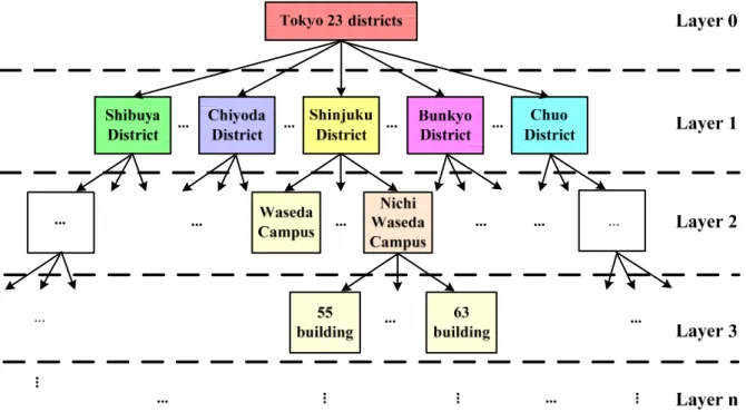
Take  the  Tokyo  23  districts  as  an  example.  Fig.  2‐1  is  the  overview  diagram  of  Tokyo  23‐districts distribution networks. According to the administrative divisions, Tokyo city can be  divided into 23 clusters at first, including the Shibuya, Shinjuku, Chiyoda, Bunkyo, Toyoshima  and other districts. If we treat the entire Tokyo as the Layer 0 of the HFD model, the 23 districts  construct the Layer 1 of the HFD model and each district is a component at Layer 1. In addition,  each  of  the  districts  can  be  subdivided  again,  according  to  the  community  structure  or  the  logical topology of the distribution networks. Takes the Shinjuku district as an example, Waseda  Campus  and  Nishi‐Waseda  Campus  are  the  components  of  the  Shinjuku  district  and  both  of  them  contain  a  number  of  load  nodes.  Meanwhile,  the  Shinjuku  district  also  contains  other  clusters just like the Waseda Campus and Nishi‐Waseda Campus, and all of clusters construct  the  Layer  3  of  the  HFD  model.  Furthermore,  the  Nishi‐Waseda  Campus  can  be  subdivided  at  Layer 4. The building of the campus is the components at this layer, for example, 55‐building,  53‐building, 63 building and so on. 

Fig.  2‐2  is  hierarchical  framework  of  Tokyo  23‐districts  distribution  networks.  In  the  framework of the Tokyo 23‐districts distribution network, the entire network is divided into n  layers. With the deeper of layer, the cluster is smaller. At the last layer, the cluster can not be  subdivided  any  more.  In  each  layer  of  the  model,  there  are  several  clusters.  Each  of  them  contains a number of load nodes. In this thesis, this kind of cluster, which contains many load  nodes, is called Load Cluster. The load cluster is the basic unit for the hierarchical fault diagnosis  model. 

  Fig. 2­2 Hierarchical framework of Tokyo 23 districts distribution networks. 

The  equation  (2.1)  is  the  complex  power  calculation  approach  for  the  Load  Cluster n  in  Layer k,  C_n^{( )k} : 

( )

( )

k

n n i

k

S =

∑

i_∈Φ S .      (2.1)  Where, the  Φ^{( )}_n^k   is the set of all the nodes in Load Cluster  C_n^{( )k} , Si is the complex power of  the Node i and the  S_n^{( )k}   is the total complex powers of Load Cluster  C_n^{( )k}   in layer k.   

In the HFD model, fault diagnosis can be carried out from the top down through the layers  to  gradually  locate  the  fault.  For  example,  we  assume  that  a  fault  occurs  at  load  cluster  “63  building” of the Fig. 2.2. Firstly, the fault can be detected at Layer 1 and located at Load Cluster 

“Shinjuku  District”  of  Layer  1.  And  then,  diagnose  the  child  load  clusters  belong  to  the  load  cluster  “Shinjuku  District”  at  the  Layer  2  and  the  fault  can  be  further  located  at  load  cluster 

“Nishi‐Waseda  Campus”.  Finally,  diagnose  the  child  load  cluster  belong  to  the  “Nishi‐Waseda  Campus” at Layer 3 and the fault can be located at “63 building”. 

The HFD model is applied to diagnose the faults have two advantages.   

1)  The  faults  location  is  gradually  located  from  the  top  of  the  hierarchical  structure  downward through the layers. It is simple and computationally inexpensive.   

The  entire  distribution  networks  contain  thousands  of  nodes.  When  a  fault  occurs  at  a  certain node, it is hard to locate the fault node from all the nodes in one time. For the HFD model,  we can locate the fault layer by layer from the top to down. In each layer, there are only several  or  dozens  of  Load  Clusters.  Compared  to  the  entire  model,  the  HFD  model  is  simpler  and  the  computation time is faster. 

2) Whatever the effect of the fault is small or large, the hierarchical model is always able to  locate the fault in final.   

In  the  standpoint  of  entire  Tokyo  23  districts  dispatching  center,  faults  can  be  classified  into 3 levels.   

a) The fault occurs at the household electricity equipment, we call it tiny level; 

b) The fault occurs at the community electricity equipment, we call it middle level; 

c) The fault occurs at the district electricity equipment, we call it large level. 

The different level of faults, have the different influence range to the dispatching center of  Tokyo.  If  a  fault  occurs  at  the  electrical  equipment  of  the  district  and  leads  to  blackout  in  a  large‐scale area, the effect of the fault is large and it is easy to be identified by the dispatching  center of Tokyo. However, if the fault is the tiny fault, due to the little influence of it, the dispatch 

center is hard to detect it.   

However,  in  our  model,  by  monitoring  the  different  layer  of  model,  whatever  the  fault  is  large or small, the fault can be detected layer by layer. For example, we can monitor the Layer 1  or lower Layer (Layer 2) to monitor the fault may be occurred at Layer 3. In this way, the fault  can be identified earlier and removed it timely, avoiding the worse impact on the network. 

2.2.2 Procedures of HFD Algorithm   

As  mentioned  above,  the  fault  diagnosis  start  from  the  top  to  down  and  locate  the  fault  position  gradually.  There  are  many  reasons  for  performing  a  fault  diagnosis.  For  example,  a  supervisor  might  want  to  know  if  it  is  safe  for  one  of  the  power  plants  in  a  large  system  to  supply power to the loads it services. In this case, diagnosis should start at the layer containing  that plant. On the other hand, for maintenance, a supervisor might need to check if there is a  fault  in  a  particular  area.  In  that  case,  the  diagnosis  should  start  at  the  relevant  layer. 

Hierarchical  fault  diagnosis  provides  the  flexibility  needed  to  handle  a  variety  of  diagnostic  needs. 

Extracting the key points from the above discussion gives us the following HFD algorithm. 

If Layer  k  is to be checked, fault diagnosis starts from that layer. 

Step 1) Construct a hierarchical model of the network and calculate the dynamic model of  each load cluster. 

Step 2) Monitor the Layer k of the hierarchical model in a real‐time fashion. If a fault occurs  at load cluster Ck, then go to the next step. 

Step 3) Go to Layer k+1 and check the child load clusters of Ck in this layer to determine  which cluster contains the  fault (Ck+1 for  example). If the cluster containing  the fault  has only  one node, go to Step N. 

Step  4)  Go  to  Layer k+2  and  examine  the  child  clusters  of Ck+1  in  this  layer  to  determine  which cluster contains the fault. If the cluster containing the fault has only one node, go to Step  N. 

…   

Step N) Determine the type of fault by analyzing the amplitude and phase of the estimated  state of the smallest cluster containing the fault, which was produced by the dynamic model. 

Note that, if a cluster containing a fault has only one node, then the location of the fault is  determined in that step and the type is determined in the next step; there is no need to always  descend to the lowest layer. Furthermore, the fault diagnosis does no need to scan all the load