JAIST Repository: Semantic Class Disambiguation for All Words

全文

(1)JAIST Repository https://dspace.jaist.ac.jp/. Title. Semantic Class Disambiguation for All Words. Author(s). Truong Vo, Huu Thien. Citation Issue Date. 2016-09. Type. Thesis or Dissertation. Text version. author. URL. http://hdl.handle.net/10119/13744. Rights Description. Supervisor:白井清昭, 情報科学研究科, 修士. Japan Advanced Institute of Science and Technology.

(2) Semantic Class Disambiguation for All Words. Truong Vo Huu Thien School of Information Science Japan Advanced Institute of Science and Technology September, 2016.

(3) Master’s Thesis. Semantic Class Disambiguation for All Words. 1410219 Truong Vo Huu Thien. Supervisor : Associate Professor Kiyoaki Shirai Main Examiner : Associate Professor Kiyoaki Shirai Examiners : Associate Professor Nguyen Le Minh Professor Satoshi Tojo. School of Information Science Japan Advanced Institute of Science and Technology August, 2016.

(4) Acknowledgement Foremost, I would first like to thank my thesis supervisor Associate Professor Kiyoaki Shirai of the Information Science at Japan Advanced Institute of Science and Technology. I am gratefully indebted for his guidance, inspiration, and support from the very beginning to the thesis accomplishment. Besides, I would like to thank the rest of my thesis committee members: Associate Professor Nguyen Le Minh and Professor Satoshi Tojo for their encouragement, valuable comments and insightful questions. During the time I conducted my research, I received several useful comments and suggestions from members in Shirai Laboratory. My most sincere thanks and wishes to all of them. I also would like to show my gratitude to JAIST, Viet Nam National University, and Japanese Government JASSO for giving me the opportunity to study, research, expense of wonderful life experiences in Japan. Last but not least, my beloved family and friends are always my strong motivation for me to overcome all of challenges I have taken on the road I passed and to come. I want to express my great appreciation to all of them for all of the support they have given. Truong Vo Huu Thien August 26, 2015. i.

(5) Contents 1 Introduction 1.1 Background and Motivation . . . . . . . . . . . . . . . . . . . . . . . . . . 1.2 Goal . . . . . . . . . . . . . . . . . . . . . . . . . . . . . . . . . . . . . . . 1.3 Organization of the thesis . . . . . . . . . . . . . . . . . . . . . . . . . . .. 1 1 2 3. 2 Related Work 2.1 Word Sense Disambiguation . . . . . . . . . . . . . . . . . . . . . . . . . . 2.2 Semantic Class Disambiguation . . . . . . . . . . . . . . . . . . . . . . . . 2.3 Discussion . . . . . . . . . . . . . . . . . . . . . . . . . . . . . . . . . . . .. 4 4 6 7. 3 Proposed method 3.1 Semantic Class . . . . . . . . . . . . . . . 3.2 Ariyakornwijit’s method . . . . . . . . . . 3.3 Proposed Architecture . . . . . . . . . . . 3.4 Features . . . . . . . . . . . . . . . . . . . 3.4.1 Local Context . . . . . . . . . . . . 3.4.2 Part of Speech . . . . . . . . . . . . 3.4.3 Collocations . . . . . . . . . . . . . 3.4.4 Syntactic Features . . . . . . . . . 3.5 Learning Algorithm . . . . . . . . . . . . . 3.6 Selection of Semantic Class . . . . . . . . . 3.7 Feature Selection . . . . . . . . . . . . . . 3.7.1 Frequency Based Feature Selection 3.7.2 Pearson’s chi-squared Test . . . . . 4 Evaluation 4.1 Test Data . . . . . . . . . . . . 4.2 Training Data . . . . . . . . . . 4.2.1 Experiment I . . . . . . 4.2.2 Experiment II . . . . . . 4.3 Results . . . . . . . . . . . . . . 4.3.1 Results of Experiment I 4.3.2 Results of Experiment II 4.3.3 Discussion . . . . . . . .. . . . . . . . .. . . . . . . . . ii. . . . . . . . .. . . . . . . . .. . . . . . . . .. . . . . . . . .. . . . . . . . . . . . . .. . . . . . . . .. . . . . . . . . . . . . .. . . . . . . . .. . . . . . . . . . . . . .. . . . . . . . .. . . . . . . . . . . . . .. . . . . . . . .. . . . . . . . . . . . . .. . . . . . . . .. . . . . . . . . . . . . .. . . . . . . . .. . . . . . . . . . . . . .. . . . . . . . .. . . . . . . . . . . . . .. . . . . . . . .. . . . . . . . . . . . . .. . . . . . . . .. . . . . . . . . . . . . .. . . . . . . . .. . . . . . . . . . . . . .. . . . . . . . .. . . . . . . . . . . . . .. . . . . . . . .. . . . . . . . . . . . . .. . . . . . . . .. . . . . . . . . . . . . .. . . . . . . . .. . . . . . . . . . . . . .. . . . . . . . .. . . . . . . . . . . . . .. . . . . . . . .. . . . . . . . . . . . . .. . . . . . . . .. . . . . . . . . . . . . .. 8 8 8 12 14 14 16 16 18 20 21 22 22 22. . . . . . . . .. 24 24 28 29 30 32 32 33 35.

(6) 5 Conclusion and Future Work 36 5.1 Conclusion . . . . . . . . . . . . . . . . . . . . . . . . . . . . . . . . . . . . 36 5.2 Future Work . . . . . . . . . . . . . . . . . . . . . . . . . . . . . . . . . . . 37. This dissertation was prepared according to the curriculum for the Collaborative Education Program organized by Japan Advanced Institute of Science and Technology and Ho Chi Minh National University. iii.

(7) List of Figures 3.1 3.2 3.3 3.4 3.5 3.6 3.7 3.8 3.9 3.10 3.11 3.12 3.13 3.14 3.15 3.16. Traditional Approach of WSD . . . . . . . . . . . . . . . . . . . . . . . . . Ariyakornwijit’s Approach [1] . . . . . . . . . . . . . . . . . . . . . . . . . Ariyakornwijit’s Architecture [1] (OVR-SCD) . . . . . . . . . . . . . . . . Example of Target Word and Its Context(1) . . . . . . . . . . . . . . . . . Proposed Architecture (PW-SCD) . . . . . . . . . . . . . . . . . . . . . . . Training Procedures . . . . . . . . . . . . . . . . . . . . . . . . . . . . . . Example of Target Word and Its Context (2) . . . . . . . . . . . . . . . . . Example of Target Word and Its Context (3) . . . . . . . . . . . . . . . . . POS feature . . . . . . . . . . . . . . . . . . . . . . . . . . . . . . . . . . . Part of Speech of “immunisation” in the Context . . . . . . . . . . . . . . An example of POS feature . . . . . . . . . . . . . . . . . . . . . . . . . . Collocation Feature . . . . . . . . . . . . . . . . . . . . . . . . . . . . . . . Example of Collocation Feature . . . . . . . . . . . . . . . . . . . . . . . . Example of Extraction of Collocation Feature from Different Target Words Example of Syntactic Feature . . . . . . . . . . . . . . . . . . . . . . . . . Support Vector Machine separators . . . . . . . . . . . . . . . . . . . . . .. 4.1 4.2. An Sample of Target Word ‘difference’ in Test Data . . . . . . . . . . . . . 25 An Sample of Target Word ‘begin’ in Test Data . . . . . . . . . . . . . . . 26. iv. 10 10 11 12 13 15 15 16 16 17 17 17 17 18 20 21.

(8) List of Tables 3.1 3.2 3.3 3.4. . 9 . 14 . 14. 3.5 3.6. List of Semantic Classes in WordNet . . . . . . . . . . . . . . . . . . . . Average Number of Samples in OVR-SCD . . . . . . . . . . . . . . . . . Average Number of Samples in PW-SCD . . . . . . . . . . . . . . . . . . Type Dependencies and Collapsed Typed Dependencies Extracted by Stanford Parser . . . . . . . . . . . . . . . . . . . . . . . . . . . . . . . . . . . Example of Majority Voting . . . . . . . . . . . . . . . . . . . . . . . . . Contingency Table of Feature and Semantic Class . . . . . . . . . . . . .. 4.1 4.2 4.3 4.4 4.5 4.6 4.7. Lexical Entry of the Noun ‘different’ . . . . . Lexical Entry of the Verb ‘begin’ . . . . . . . List of Target Word . . . . . . . . . . . . . . . Statistics of Training Data in Experiment I . . Statistics of Training Data in Experiment II . Accuracy of Semantic Class Disambiguation in Accuracy of Semantic Class Disambiguation .. . . . . . . .. v. . . . . . . . . . . . . . . . . . . . . . . . . . . . . . . . . . . . Experiment . . . . . . .. . . . . . I .. . . . . . . .. . . . . . . .. . . . . . . .. . . . . . . .. . . . . . . .. . . . . . . .. . . . . . . .. . 19 . 22 . 23 27 27 28 30 31 33 34.

(9) Chapter 1 Introduction 1.1. Background and Motivation. Word Sense Disambiguation (WSD) is a task to identify a sense of a word in a given context when the word has multiple meanings. Unlike human brain which is quite proficient at recognizing the correct meaning of a word in a sentence, the computer scientist faces a serious problem to develop word sense disambiguation ability for computers that can interact with human. To illustrate how WSD is performed, let’s consider an example below. The word ‘bank’ in the dictionary1 has two senses: 1. A raised shelf or ridge of ground; a long, high mound with steeply sloping sides; one side or slope of such a ridge or mound. 2. The shop, office, or place of business of a money changer or moneylender. There are two example sentences containing the target word ‘bank’: 1. The boy leapt from the bank into the cold water. 2. I have money in the bank. It is not difficult for human to realize the word “bank” in the first sentence has the first sense and in the second sentence it has the second sense. WSD is a method to replicate this incredible human ability into the computers. WSD plays an important role in Natural Language Processing (NLP). It is one of the fundamental techniques used for many NLP applications such as machine translation, information retrieval, and opinion mining. It is also considered as one of the oldest problems in the early day of machine translation formulated in the 1940s. Therefore, many approaches have been proposed to solve this problem: a dictionarybased method that uses lexical resources containing glosses or definition sentences of the word senses, supervised machine learning based method that uses a manually sense 1. http://www.oxfordlearnersdictionaries.com/. 1.

(10) tagged corpus as the training data, and an unsupervised learning based method that trains a classifier of WSD from unannotated text. Recently, supervised machine learning shows the best performance among various approaches for WSD. However, supervised learning requires a considerable amount of training data, i.e. a collection of texts annotated with the gold senses of the words. Since manual annotation of the senses requires much cost and time, it is often difficult to prepare enough data for training. This problem is known as “Knowledge Acquisition Bottleneck” problem or “Data Sparseness” problem. Mihalcea and Chklovski estimated that it took 80 years for a person to manually build labeled training data for 20,000 words in a common English dictionary [15]. In the ordinary approaches of WSD, a classifier is trained for each target word, since sense inventory is unique to the target word. It is necessary to train many WSD classifiers to disambiguate the senses of all words in the text, however, it is difficult to prepare the annotated training data for all words, especially for the low frequent word. On the other hand, an alternative approach was proposed to tackle this problem. In this approach, a set of semantic classes is used as a common sense inventory for all words. The semantic class refers to an abstract concept of the words, such as ‘plant’, ‘shape’, and ‘time’. Instead of training individual classifiers for the target words, the universal classifiers that can determine the semantic class of any words including the low frequent word are trained. It can alleviate knowledge acquisition bottleneck problem, since a small number of the classifiers are required to train. As the semantic class only expresses more general concept than the sense, semantic class disambiguation (a coarse grained WSD in other words) is insufficient for some NLP applications such as machine translation. However, it is obviously useful for many applications, such as information retrieval and acquisition of domain knowledge [18]. To understand how useful Semantic Class Disambiguation (SCD) is in information retrieval, we can consider an example of the word ‘apple’ containing 3 senses: apple as a fruit, apple as a tree and apple as a company. A correct disambiguation of the word ‘apple’ in the query sentence and the sentences in a document collection improves the performance of information retrieval system. When a user want to search the information about a product of Apple company, the semantic class disambiguation can prevent the system from retrieving irrelevant documents about apple fruit and apple tree. Moreover, SCD is successfully applied in CRYSTAL [22], which can surpass human intuition in creating reliable information extraction rules.. 1.2. Goal. This paper proposes a novel method to disambiguate the semantic classes of all words. In the previous method of semantic class disambiguation, the training data often consists of imbalanced positive and negative samples. The system trained from such data tends to classify a new input into the majority class. It causes decline of performance of semantic class disambiguation. Our new architecture enables us to train the classifiers from more balanced training data. 2.

(11) The dimension of feature vector in this method is very high. Using all of features might not be good because some of them are noisy and decrease the performance. Various techniques to choose the important features, called feature selection, was proposed to improve the performance of supervised learning. In this research, 2 feature selection techniques are used and empirically evaluated: frequency based method and Pearsons chi-squared test.. 1.3. Organization of the thesis. The rest of the thesis is organized as follows: • Chapter 2 introduces related work and clarifies the originally of the proposed method. • Chapter 3 describes our new method for semantic class disambiguation. • Chapter 4 reports results of an experiment to evaluate our method. • Finally, Chapter 5 concludes the paper and discusses future work.. 3.

(12) Chapter 2 Related Work In this chapter, we introduce essential knowledge of word sense disambiguation and some previous approach on semantic class or coarse grained word sense disambiguation.. 2.1. Word Sense Disambiguation. First, we explain more precise definition of word sense disambiguation (WSD). The senses of a word is defined by a dictionary or lexical database. It is generally called ‘sense inventory’. WSD is a task to choose the appropriate sense of a target word in a given context from the senses of the target word in the sense inventory. Here ‘target word’ refers to a word whose sense is aimed at being disambiguated. Obviously, the target word is an ambiguous word that has two or more senses in the sense inventory. The input of the WSD is the target word in a certain context (sentence, paragraph or document) as well as the sense inventory, and the output is one of the senses of the target word in the sense inventory. There are two major tasks in WSD: lexical sample task and all words task. • Lexical sample: is a task to disambiguate a small sample of the target words. • All words: is a task to disambiguate all the words in the text. All words task is more difficult than the lexical sample task. When the supervised learning is applied to the lexical sample task, a collection of the sentences that includes the gold senses for a limited number of the target words is required. On the other hand, a sense tagged corpus that contains the gold senses of all words is required for all words task, which requires much costs to construct. The difficulty and significance of WSD problem was recognized and understood by machine translation researchers in late 1940s. After that, large-scale lexical database and resources useful for WSD, such as the Oxford Advanced Learner’s Dictionary of Current English (OALD) [7], were built. Several researchers investigated knowledge based and dictionary based methods, which utilized the information derived from the lexical database for word sense disambiguation. However, the performance of them is not actually as high as expectation. Next, machine learning techniques are highlighted in the field of natural 4.

(13) language processing. Because many tasks in NLP can be regarded as a classification problem for which machine learning can be applicable. WSD is also a problem that supervised learning has been successfully applied. There are two major approaches for WSD: deep approach and shallow approach. • Deep approach: assumes that we have comprehensive knowledge. For instance, we suppose to have knowledge “you have money in place of business of a money changer or moneylender, not in a long, high mound with steeply sloping sides.” We can choose the appropriate sense of the target word ‘bank’ using this knowledge. However, such common sense knowledge is very hard to describe in a computer readable format. It is also hard to accumulate comprehensive knowledge in the world. Therefore, the deep approach is not successful in real applications. • Shallow approach: only considers surrounding words of the ambiguous word instead of trying to understand the context precisely. In theory, the shallow approach might not as powerful as the deep approach, but it performs much better in practice due to the limitation of computational power. Hence, many researchers take shallow approaches for WSD. The most of conventional approaches for WSD can be categorized into the following four methods [19]. • Dictionary-based and Knowledge-based methods : This technique explores dictionary, thesauri, and lexical knowledge without using any corpus to disambiguate the senses of the word. Banerjee and Pedersen presented a new measure of semantic similarity between concepts that is based on the overlaps in their glosses in a dictionary [2]. The research showed the new measure was effectively applied for word sense disambiguation. • Semi-supervised methods or minimal supervised methods: This utilizes both label and unlabel data. Because the lack of labeled data, many previous researches tend to use this approach. This approach uses a small annotated corpus as a seed data in a boostrapping process. Mihalcea and Faruque introduced a minimal supervised sense tagger, called SenseLearner, which can disambiguate all content words in a text using WordNet [17]. This method used SemCor, a sense annotated corpus, as the training data to learn a WSD model for the words in SemCor corpus, while a memory based learner was applied to train another model for WSD of unseen words in SemCor corpus by generalizing the words under syntactic relations as training samples. The method achieved 64.6 % of an average accuracy. • Supervised methods: Machine learning algorithms are used for training WSD classifiers from sense tagged corpora. • Unsupervised methods: This technique works mostly on a raw corpora with assumption that similar senses appear in similar contexts. Hence, they can induce word sense from unlabeled text by clustering word occurrences and classify 5.

(14) the occurrences of a new word into the induced cluster. A novel approach was recently proposed by Bordag which performed word sense induction based on word triplets [3]. This method was based on “one sense per collocation” assumption and clustered triplets of words instead of pairs using sentence co-occurrences as features. The shallow approaches using supervised learning show the advantage; it surpasses other approaches in performance. In recent research, Support Vector Machines [11] is the most successful approaches because it may be able to handle high dimensionality of feature space which is usually huge in WSD. However, supervised method faces a knowledge acquisition bottleneck because it depends on a large manually sense tagged corpora which consume huge cost and time.. 2.2. Semantic Class Disambiguation. As described above, the senses of the target word are defined by a dictionary. The dictionary also defines granularity of the senses from a coarse to fine grained senses. The coarse grained senses represent board meanings, while the fine grained senses distinguish subtle difference of the meaning. In fact, the disambiguation of the coarse grained sense is easier than the fine grained sense. Human is also better at WSD in coarse grained level than fine grained level. Furthermore, even the coarse grained sense disambiguation is useful for some NLP applications such as information retrieval. Hence, some research tried coarse grained distinction for evaluation. Using broader distinction also helps to alleviate the knowledge acquisition bottleneck problem in supervised learning techniques. The semantic class or coarse grained word sense can be defined in various ways in previous approaches. Resnik proposed a method to build a set of conceptual classes for word senses using selectional preferences [21]. His method can automatically acquire linguistic predicate constraints from a raw corpus. Although his method was evaluated on fine-grained word disambiguation, coarse-grained WSD could apply his association scores for conceptual classes. Levin proposed a method for English verb classification [12]. Supposing that a meaning of a verb influences its syntactic behavior, she defined a set of coherent verb classes and their alternations based on their syntactic behavior. This classification of the English verbs can be considered as a verb inventory. Although Levin’s inventory is useful, it is based on syntactic properties unlike those in WordNet [6]. Korhonen proposed a mapping method from WordNet entries into Levin’s classes [10]. The accuracy of this method was 81% when automatically mapping 1,616 synsets arranged into hierarchy in WordNet to one of 32 Levin’s classes. Although there are a lot of work on word sense disambiguation, disambiguation of the semantic classes was not paid attention so much. Nevertheless, a few studies of semantic class disambiguation have been devoted. Izquierdo et al. presented a method to select Base Level Concepts (BLC) based on basic structural properties of WordNet [8]. Two different sets of BLC were derived by 6.

(15) considering 1) all types of relations in WordNet and 2) only the hyponymy relations. A naive classifier that chose the most frequent concept could perform a semantic tagging with 75% accuracy. Kohomban and Lee proposed a method for WSD using general concepts [9]. Intuitively, the coarse grained WSD is an easier task than the fine grained WSD. To improve the performance, their method first performed the coarse grained WSD, then the chosen coarse sense was mapped to the fine grained sense using simple heuristics. The classifier was trained by memory-based learner using four useful features: local context, part-ofspeech, collocation, and syntactic relation. They reported the accuracy reached over 77%. The most important related work of this thesis is Ariyakornwijit and Shirai’s method [1]. Using four features presented in [9] with some modification, they trained a binary classifier for each semantic class that could judge if any given word in the context had the semantic class or not. Note that the number of the trained classifiers is much less than in the previous approach. In the ordinary WSD studies, one classifier is trained for each target word, while one classifier is trained for each semantic class in Ariyakornwijit’s method. Furthermore, they used the sentences including monosemous words, which has only one semantic class, as the training data. It enabled us to prepare the training data without manual annotation. Their method achieved 28.6% of exact match accuracy and 53.0% of partial match accuracy, which far surpassed the baseline. The details of this work are introduced in Section 3.2.. 2.3. Discussion. Although Ariyakornwijit approach is promised to alleviate knowledge acquisition bottleneck since it requires much less trained classifiers than traditional WSD approach, the performance of the semantic class disambiguation of this method is still insufficient. They discussed that one of the reasons was imbalance of the positive and negative samples in the training data. This paper proposes a new architecture for semantic class disambiguation to tackle this problem. Considering semantic class disambiguation, although many definitions of the coarse grained senses or semantic classes of the words have been proposed, there seems no universal set of semantic classes for all words. The appropriate set of the semantic classes may depend on the NLP applications. In this study, the semantic classes are defined based on WordNet. However, any semantic classes can be applicable in our method. Moreover, it is useful to apply additional techniques such as feature selection and parameter optimization for improving the performance of the system. Since the feature space is huge and noisy, two feature selection methods, Pearsons chi-square test and frequency based feature selection, are experimented to reduce feature dimension. Although the feature selection is commonly used for various tasks in NLP, Ariyakornwijit and Shirai did not use it for semantic class disambiguation. This thesis reports the first attempt to investigate the effectiveness of the feature selection in the task of semantic class disambiguation.. 7.

(16) Chapter 3 Proposed method This chapter presents our proposed method and its advantages comparing to previous approach.. 3.1. Semantic Class. In this study, WordNet [6] is used as an inventory of the semantic classes. WordNet is a famous lexical database for English, which is widely used as the sense repository in many WSD researches. It groups 155,287 words into 117,659 sets of synonyms, called synsets. The synsets composes a hierarchical structure where the synsets are connected by hypernym or other semantic relations. At the top level, WordNet defines 45 unique beginners of all synsets, which are considered as the coarsest senses. We define them as a set of the semantic classes. It consists of 26 semantic classes for noun, 15 for verb, 3 for adjective and 1 for adverb. In this research, only nouns and verbs are considered for disambiguation of the target word because semantic classes of adjectives and adverbs rarely appear in the training corpus. A list of all semantic classes of the nouns and verbs with their identification number, name and definition is shown in Table 3.1.. 3.2. Ariyakornwijit’s method. This section describes more details of Ariyakornwijit’s method for semantic class disambiguation [1]. Fig. 3.1 and Fig. 3.2 show the traditional approaches and Ariyakornwijit’s approach for WSD, respectively. In most WSD studies, the sense inventory is peculiar to the target word. In Figure 3.1, the set of the senses {S11 , · · · S1n } of the target word w1 and the set of the senses {S21 , · · · S2n } of the target word w2 are different. Therefore, a bulk of WSD classifiers are trained, where each classifier selects one sense from the sense inventory for the target word in the given context. On the other hand, in Ariyakornwijit’s approach, the only one sense inventory {SC1 , . . . , SCn } that is common to all target words is defined, where SCi. 8.

(17) Id 03 04 05 06 07 08 09 10 11 12 13 14 15 16 17 18 19 20 21 22 23 24 25 26 27 28 29 30 31 32 33 34 35 36 37 38 39 40 41 42 43. Table 3.1: List of Semantic Classes in WordNet Name Definition noun.Tops unique beginner for nouns noun.act nouns denoting acts or actions noun.animal nouns denoting animals noun.artifact nouns denoting man-made objects noun.attribute nouns denoting attribute of people and objects noun.body nouns denoting body parts noun.cognition nouns denoting cognitive processes and contents noun.communication nouns denoting communicative processes and contents noun.event nouns denoting natural events noun.feeling nouns denoting feelings and emotions noun.food nouns denoting foods and drinks noun.group nouns denoting grouping of people or object noun.location nouns denoting spatial position noun.motive nouns denoting goals noun.object nouns denoting natural object (not man-made) noun.person nouns denoting people noun.phenomenon nouns denoting natural phenomena noun.plant nouns denoting plants noun.possession nouns denoting possession and transfer of possession noun.process nouns denoting natural processes noun.quantity nouns denoting quantities and units of measure noun.relation nouns denoting relations between people or things or ideas noun.shape nouns denoting two and three dimensional shapes noun.state nouns denoting stable states of affairs noun.substance nouns denoting substances noun.time nouns denoting time and temporal relations verb.body verbs of grooming, dressing and bodily care verb.change verbs of size, temperature change, intensifying, etc. verb.cognition verbs of thinking, judging, analyzing, doubting verb.communication verbs of telling, asking, ordering, singing verb.competition verbs of fighting, athletic activities verb.consumption verbs of eating and drinking verb.contact verbs of touching, hitting, tying, digging verb.creation verbs of sewing, baking, painting, performing verb.emotion verbs of feeling verb.motion verbs of walking, flying, swimming verb.perception verbs of seeing, hearing, feeling verb.possession verbs of buying, selling, owning verb.social verbs of political and social activities and events verb.stative verbs of being, having, spatial relations verb.weather verbs of raining, snowing, thawing, thundering. 9.

(18) Figure 3.1: Traditional Approach of WSD. Figure 3.2: Ariyakornwijit’s Approach [1] stands for the semantic class. For any words in the text, the appropriate semantic classes are chosen from the common sense inventory. The procedures to disambiguate the semantic class of the word are as follows. First, for each semantic class SCi , the classifier CLi is learned from the training data. CLi is a binary classifier that judges if the target word in the given context has the semantic class SCi or not. Monosemous words, which have only one semantic class, in a large corpus are used as the training data. To train CLi , the monosemous words of SCi are used as positive samples, while the monosemous words of the other semantic classes are used as negative samples. Then, for a given text, the semantic classes of the target words are determined in the following three steps. These steps are illustrated in Fig. 3.3.. • The input text is preprocessed. First, part-of-speech (POS) tagging is performed to determine POSs of the target word and the words in the context. Next, lemmatiza10.

(19) tion is performed to convert the inflected word to base form 1 . We use NLTK POS tagger and NLTK WordNet Lemmatizer [13]. • By looking up WordNet, all possible candidates of the semantic classes of the target word are obtained. In the example of Figure 3.3, three semantic classes SC1 , SC2 and SC3 are chosen. In general, it is a subset of all semantic classes. • For each candidate of the semantic class SCi , the binary classifier is applied to judge if SCi is appropriate for the target word in the given text. For classification, the features are derived from the context of the target word. • Finally, the system chooses a set of semantic classes whose corresponding classifiers judge as ‘yes’. Note that the system selects one or more semantic classes for one target word.. Figure 3.3: Ariyakornwijit’s Architecture [1] (OVR-SCD) Figure 3.4 is an example of how the system works to disambiguate a target word “treat” in a context. Five candidate semantic classes of “treat” are verb.body, verb.change, verb.cognition, verb.communication and verb.social. The classifier for verb.body will judge if the target word has this semantic class. The classifer for other semantic classes will be also applied. These classifiers make a decision with respect to features extracted from the context of the target word. Finally, the system will output all of the semantic classes judged as ‘yes’ by the classifiers. When the classifier of verb.communication judges as ‘yes’ and other classifiers judge as ‘no’, only verb.communication is chosen as the semantic class of “treat”. The number of classifiers in Ariyakornwijit’s method is equal to the total number of the semantic classes, which is much less than the traditional WSD approach where the classifiers are trained for every word. It can alleviate the data sparseness problem. Furthermore, the use of monosemous words as the training data is a promising way to create a large amount of the training data, since no manual annotation is required. However, it 1. In [1], lemmatization is not applied as preprocessing. In our implementation of Ariyakornwijit’s method in the experiment in Chapter 4, lemmatization is also applied.. 11.

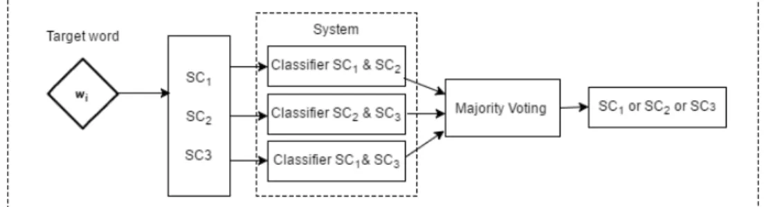
(20) Context: Is it criticism ? There is a massive amount of writing about art , only some of which can immediately be identified by a reader as criticism . Writing by the art critic of a newspaper is self - evidently criticism , in parallel with the writing of music and theatre critics ; an exhibition can be treated almost in the same way as a performance . Articles in magazines are less certainly described as criticism , for their main topics may be personalities or history , and art may be only a small part of the writers ’ account . Books and catalogues may contain criticism ; but their writers may think of themselves as art historians , philosophers , aestheticians , anthropologists , historians or biographers , and there are many other possibilities ; their books may never be identified as art criticism . Figure 3.4: Example of Target Word and Its Context(1) is rather uncertain that the monosemous words are useful for classification of ambiguous words. Because the words in the training data (monosemous word) are totally different from the target word (polysemous or ambiguous word). Such gaps may cause negative influence on semantic class disambiguation. Hereafter, we call Ariyakornwijit’s method as One-versus-rest Semantic Class Disambiguation or OVR-SCD.. 3.3. Proposed Architecture. In OVR-SCD, the monosemous words of one semantic class are used as the positive samples, and the monosemous words of all other semantic classes are used as the negative samples. It causes serious imbalance between the positive and negative samples, i.e. the number of negative samples is much greater than that of the positive samples. Such imbalance may cause decline of the performance of semantic class disambiguation, since the trained classifiers tend to almost always classify the target word as negative. To overcome this problem, we proposed a new architecture shown in Figure. 3.5. In our approach, a binary classifier is trained for each pair of the semantic class SCi and SCj . It chooses one of two semantic classes for the given target word. If the target word has three or more potential semantic classes, the classifiers of all possible pairs are applied. The detail procedures to disambiguate the semantic class of the target word are as follows: • Part-of-speech (POS) Tagging and lemmatization are performed as preprocessing. • By looking up WordNet, all possible candidates of the semantic classes of the target word are obtained. • For all pairs of the possible semantic classes, the classifiers are applied to judge if the target word has either semantic class. When SC1 , SC2 and SC3 are obtained as the potential semantic classes in Figure 3.5, pairs of (SC1 ,SC2 ), (SC2 ,SC3 ) and (SC1 ,SC3 ) are considered. 12.

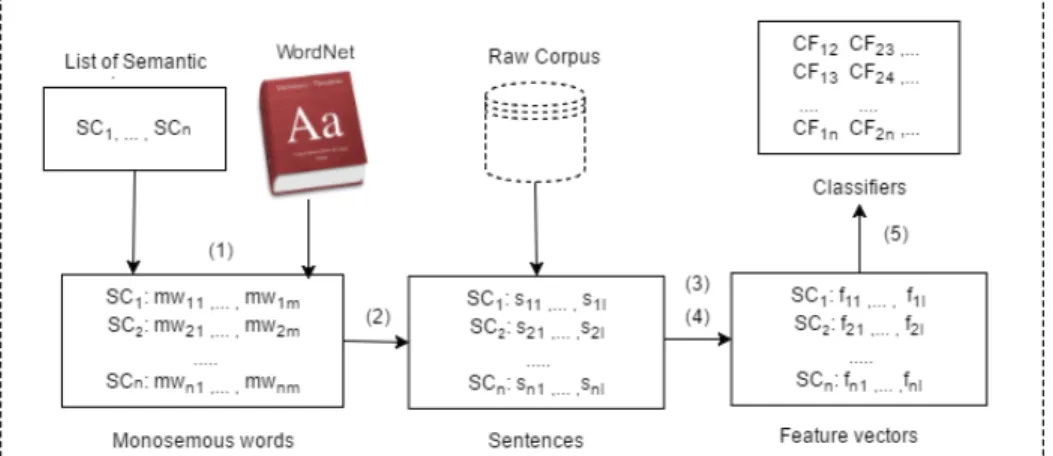
(21) • Finally, from the results of these classifiers, the final output is chosen by a simple weighted majority voting. The detail of the majority voting will be explained in Section 3.6.. Figure 3.5: Proposed Architecture (PW-SCD) Let us review the example in Figure 3.4. The target word “treat” has 5 semantic classes: verb.body, verb.change, verb.cognition, verb.communication and verb.social. In our method, a classifier is trained for each pair of the semantic classes. The possible pairs of the semantic classes are shown below2 . (body,change), (body,cognition), (body,communication), (body,social), (change,cognition), (change,communication), (change,social), (cognition,communication), (cognition, social), (communication,social) Therefore, 10 classifiers are trained. The classifiers choose either of two semantic classes. The final output is chosen from the results of these 10 classifiers by the majority voting, which will be described later. The advantage of this approach is that the positive and negative samples in the training data can be well balanced. For the pair of SCi and SCj , the positive and negative samples are the monosemous words of SCi and SCj , respectively. The number of the monosemous words of two semantic classes is expected to be comparable. The disadvantage is that the number of the classifiers is more than OVR-SCD. However, it is much less than the traditional WSD where the classifiers should be trained for all target words. Hereafter, we call this architecture Pair-wise Semantic Class Disambiguation (PW-SCD). Table 3.2 and 3.3 show statistics of OVR-SCD and PW-SCD, respectively. They show an average of the number of each positive and negative sample for the semantic class disambiguation classifiers, in terms of each noun and verb. The statistics are obtained from the Daily Yomiuri corpus [5], which is used in the experiment in Chapter 4. In statistics of PW-SCD, the fewer semantic class is regarded as the positive class in each pair-wise classifier. We can find excessive imbalance in OVR-SCD in Table 3.2. On the other hand, seeing Table 3.3, the number of two kinds of the training samples can be balanced better in our PW-SCD. 2. The prefix ‘verb.’ is omitted.. 13.

(22) Table 3.2: Average Number of Samples in OVR-SCD POS Positive Negative Noun. 126,595. 1,250,593. Verb. 61,833. 865,669. Table 3.3: Average Number of Samples in PW-SCD POS Positive Negative Noun. 69,833. 172,860. Verb. 27,728. 70,113. The procedures to train the semantic class disambiguation classifiers are shown in Figure 3.6. It consists of the following 5 steps. (1) For each semantic class SCi , a list of the monosemous word (mwij ) of SCi is retrieved from WordNet. (2) From a large raw corpus, the sentences (sij ) including the monosemous word of SCi are retrieved. For each monosemous word in the sentences, SCi is annotated as the gold semantic class. (3) Preprocessing is performed on the retrieved sentences. It consists of POS tagging and lemmatization. We use NLTK POS tagger and NLTK WordNet Lemmatizer [13]. (4) From each monosemous word and its context, the features for machine learning are extracted. Thus we can obtain the instances of SCi represented as the feature vectors (fij ). (5) For each pair of the semantic class SCi and SCj , the classifier CLij , which judges if the word has either SCi or SCj , is trained from the feature vectors of SCi and SCj .. 3.4. Features. We use the exactly same features in Ariyakornwijit’s method [1]. It consists of four features. These features are widely used for WSD task.. 3.4.1. Local Context. Local context is represented by the words around the target word. It is so called Bagof-words feature. The words in a context window whose size is Nc are extracted as the features, i.e. Nc words to the left and Nc words to the right of the target word. Precisely, 14.

(23) Figure 3.6: Training Procedures lemmatized form of the content words are extracted in the context window as the local context feature. Note that the local context features are extracted from the sentence including the target word, that is, not extracted beyond the sentence boundary. Function words, punctuation and number are not extracted. An parameter of this feature is the size of the context window Nc . In the experiment, Nc was set as 5 since it worked fairly well with a small sample of data in a preliminary experiment. Let us consider an example in Figure 3.4 where the target word is “immunisation” to explain how to extract the local context feature. Context: After immunisation you must wait at least one month before becoming pregnant. Eat properly Eating well before and during pregnancy is very important. It keeps you fit and helps you to have a healthy baby. You don’t need a special diet and eating for two could mean you put on too much weight. Figure 3.7: Example of Target Word and Its Context (2) The local features when the window size Nc = 5 are ‘after’, ‘must’, ‘wait’, ‘least’, ‘one’ and ‘month’. Let us consider another example in Figure 3.8 where the target word is “add”.. 15.

(24) Context: Very often they are pleased to invite ACET in as a church - based agency . Our educators present a personal message , each one having had experience of caring for those dying with AIDS at home . Furthermore our work in Uganda and Romania adds a wider perspective . The content of each lesson is agreed beforehand in consultation with teachers so it can be tailored to the priorities and individual needs of the school or class . Prejudices are challenged and myths exposed for example that only homosexual men and drug users are at risk . Figure 3.8: Example of Target Word and Its Context (3) In this example, the local features when the window size Nc = 5 are ‘romania’, ‘wider’, ‘Uganda’, ‘perspective’, ‘work’, ‘furthermore’, ‘content’, ‘home’, ‘lesson’, and ‘agreed’. 3.4.2. Part of Speech. POS feature is 2-gram, 3-gram and 4-gram of the parts-of-speech including the target word. Since the monosemous words are used, the target words that have the semantic class SCi are different in the training samples. Thus POSs of the target words are also different. Therefore, the POS of the target instance is always represented by the special character ‘T’, which refers to a wildcard matching any target instance. POS features can be represented as Figure 3.9. 2-gram: {p−1 T }, {T p−1 } 3-gram: {p−2 p−1 T }, {p−1 T p1 }, {T p1 p2 } 4-gram: {p−3 p−2 p−1 T }, {p−2 p−1 T p1 }, {p−1 T p1 p2 } {T p1 p2 p3 } Figure 3.9: POS feature In this figure, p1 , p2 , and p3 are POSs of 1,2,3 words after the target word respectively. Similarly, p−1 , p−2 , and p−3 are POSs of 1,2,3 words before the target word. When there are not enough words to either side of the target word, the value ‘NULL’ is used to fill the vacancies. To illustrate how POS features are extracted, we consider the example of Figure 3.7. Figure 3.10 shows POSs of all words in the context of the target word ‘immunisation’. Note that each word is separated by ‘/’, where the left is the word and the right is its POS. Then POS features are extracted as Figure 3.11.. 3.4.3. Collocations. Collocation is a sequence of the words consisting of the target word and its surrounding words. In this research, 2-gram, 3-gram, and 4-gram of the words including the target 16.

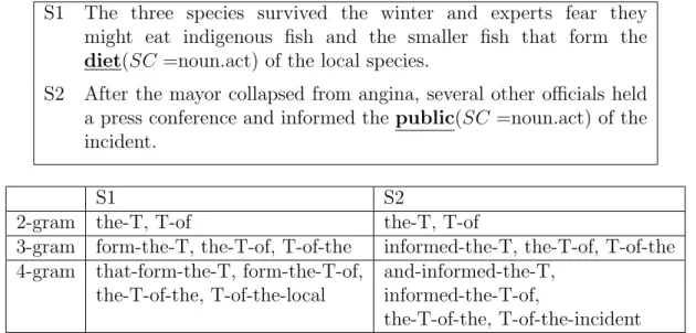
(25) After/IN immunisation/NN you/PRP must/MD wait/VB at/IN least/JJS 1/CD month/NN before/RB becoming/VBG pregnant/JJ ./. Eat/NNP properly/RB Eating/NNP well/RB before/IN and/CC during/IN pregnancy/NN is/VBZ very/RB important/JJ ./. It/PRP keeps/VBZ you/PRP fit/VBP and/CC helps/NNS you/PRP to/TO have/VB a/DT healthy/JJ baby/NN ./. You/PRP do/VBP n‘t/RB need/VB a/DT special/JJ diet/NN and/CC eating/VBG for/IN two/CD could/MD mean/VB you/PRP put/VB on/RP too/RB much/JJ weight/NN ./. Figure 3.10: Part of Speech of “immunisation” in the Context 2-gram: {IN T}, {T PRP} 3-gram: {NULL IN T}, {IN T PRP}, {T PRP MD } 4-gram: {NULL NULL IN T}, {NULL IN T PRP}, {IN T PRP MD} {T PRP MD VB} Figure 3.11: An example of POS feature instance itself are extracted as the collocation feature. Similar to the POS feature, the target instance is replaced with the wildcard symbol ‘T’. The collocation feature can be represented as Figure 3.12. w0 is the target word. w1 , w2 , and w3 are 1,2,3 words after the target word respectively. Similarly, w−1 , w−2 , and w−3 are 1,2,3 words before the target word. Similar to Part of Speech feature, symbol “NULL” will be filled the vacancies if there is not enough words on each side. 2-gram: {w−1 T}, {T w−1 } 3-gram: {w−2 w−1 T}, {w−1 T w1 }, {T w1 w2 } 4-gram: {w−3 w−2 w−1 T}, {w−2 w−1 T w1 }, {w−1 T w1 w2 } {T w1 w2 w3 } Figure 3.12: Collocation Feature From the example shown in Figure 3.7, 2-gram, 3-gram and 4-gram of collocation feature are extracted as shown in Figure 3.13. 2-gram: {after T}, {T you} 3-gram: {null after T}, {after T you}, {T you must} 4-gram: {null null after T}, {null after T you}, {after T you must}, {T you must wait} Figure 3.13: Example of Collocation Feature. 17.

(26) To illustrate how the wildcard ‘T’ works, we show another example in Figure 3.14. Let us suppose there are two sentences S1 and S2 in the training data. Both ‘diet’ and ‘public’ are monosemous words that have only one semantic class ‘noun.act’. Thus these sentences can be used for training the classifier that judges if the target word has ‘noun.act’ or the other semantic class. Collocation features are extracted from S1 and S2 as shown in the bottom table in Figure 3.14. Note that several same features are extracted from these sentences, such as ‘the-T-of-the’ and ‘the-T-of’ and so on. The feature ‘the-T-of-the’ indicates that the semantic class ‘noun.act’ can be appeared in the context where the preceding word is “the” and the succeeding words are “of the”. If the target word is not represented by ‘T’, the different features will be extracted, failing to capture the similarity between these two training samples. By replacing the target word with the common symbol ‘T’, the exactly same features can be extracted from S1 and S2. S1. The three species survived the winter and experts fear they might eat indigenous fish and the smaller fish that form the diet(SC =noun.act) of the local species.. S2. After the mayor collapsed from angina, several other officials held a press conference and informed the public(SC =noun.act) of the incident.. 2-gram 3-gram 4-gram. S1 the-T, T-of form-the-T, the-T-of, T-of-the that-form-the-T, form-the-T-of, the-T-of-the, T-of-the-local. S2 the-T, T-of informed-the-T, the-T-of, T-of-the and-informed-the-T, informed-the-T-of, the-T-of-the, T-of-the-incident. Figure 3.14: Example of Extraction of Collocation Feature from Different Target Words. 3.4.4. Syntactic Features. Syntactic feature is direct grammatical relation between the target word and its surrounding word, such as subject-verb, object-verb and noun-adjective. It is well known that the words connected to the target words via syntactic relation are useful for WSD. Thus syntactic relation is one of the conventional feature for WSD. First, the sentence is parsed by Stanford Parser [14]. Only the sentence containing the target word is analyzed. Stanford Parser offers two kinds of dependencies: typed dependencies and collapsed typed dependencies. • Typed Dependencies: are representation where each word in the sentence (except the head of the sentence) is independently treated to the other word.. 18.

(27) • Collapsed Typed Dependencies: are constructed by collapsing a pair of typed dependencies into a single typed dependency, whose name is abbreviated based on the word between two dependencies. Table 3.4 shows the types dependencies and collapsed typed dependency from the sentence After immunisation you must wait at least 1 month before becoming pregnant. , which is the sentence including the target word in the example of Figure 3.7. Note that two relations of “prep(wait-5,After-1)” and “pobj(After-1,immunisation-2)” in types dependencies are merged into one relation “prep after(wait-5,immunisation-2)” in collapsed typed dependencies. The relations “prep(wait-5,before-10)” and “pcomp(before10,becoming-11)” are collapsed as “prep before(wait-5,becoming-11)”, too. Table 3.4: Type Dependencies and Collapsed Typed Dependencies Extracted by Stanford Parser Stanford Sparser Typed Dependencies Collapsed Typed Dependencies prep(wait-5, After-1) prep after (wait-5, immunisation-2) pobj(After-1, immunisation-2) nsubj(wait-5, you-3) nsubj(wait-5, you-3) aux(wait-5, must-4) aux(wait-5, must-4) root(ROOT-0,wait-5) root(ROOT-0, wait-5) quantmod(1-8, at-6) quantmod(1-8, at-6) mwe(at-6, least-7) mwe(at-6, least-7) dobj(wait-5, 1-8) dobj(wait-5, 1-8) tmod(wait-5, month-9) tmod(wait-5, month-9) prep before(wait-5, becoming-11) prep(wait-5, before-10) acomp(becoming-11, pregnant-12) pcomp(before-10, becoming-11) acomp(becoming-11, pregnant-12) In this research, we use collapsed typed dependencies to represent syntactic feature. Stanford Parser produces a set of collapsed typed dependency in the form of ‘rel(w1 , w2 )’ or ‘abbreviated relation name(governor, dependent)’, where w1 is governor and w2 is dependent under the relation ‘rel’. When the dependency including the target instance is extracted, it is replaced by the wildcard symbol ‘T’. That is, rel(w1 , T ) and rel(T, w2 ) are extracted as the syntactic feature. All of word indices in governor and dependent are removed. Finally, Figure 3.15 shows all the syntactic features extracted from the example of Table 3.4.. 19.

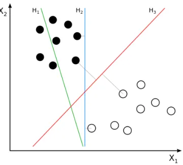
(28) prep after(wait, T), nsubj(wait,you), aux(wait, must),root(ROOT, wait), quant-mod(1, at), mwe(at, least), dobj(wait, 1), tmod(wait, month), prep before(wait, becoming), acomp(becoming, pregnant) Figure 3.15: Example of Syntactic Feature. 3.5. Learning Algorithm. In this research, Support Vector Machine (SVM) [4] is chosen as an algorithm for classification. SVM is a supervised learning which effectively analyzes and classifies patterns on high-dimensional feature space. SVM is a binary classifier, that is, the number of the classes are two. They are often called as positive and negative classes. In classification, SVM makes a good separation by constructing a hyperlane that separates the positive and negative samples in the training data and has the largest distance between to the nearest training data points (also called functional margin). The points that are closest to the separating hyperplane are called as support vectors. The idea is based on the fact that the larger the margin is, less classification errors is found. Figure 3.16 3 illustrates how the largest functional margin can optimize the classification. The black and white points stand for the positive and negative samples, respectively. As we can see, the separator H1 cannot separate the data of two classes. H2 can separate the positive and negative samples, but it is not very good since the margin is small. If an unknown positive (or negative) data point is located near the positive (or negative) support vector, its position is likely to be in the area of negative (or positive) side, causing classification error. H3 shows the best separation with the largest margin. Because an unknown data near the support vector is more likely to be located in the area of the same orientation side. In this research, the classifier will work as follows: (1) First, the training data for each semantic class is prepared. (2) Then, the model will be built using the SVM algorithm. (3) The test data will be classified by the trained model. (4) The semantic class which is the most likely for the target word will be chosen as the output. In the experiment, Sklearn library [20] is used to train SVM classifiers. SVM in Sklearn uses a kernel function to transform data in raw representation to feature vector representation. The kernel we use is the Gaussian radial basis function. There are two parameters in Sklearn library: gamma and C. In this research, they are set as the default setting, i.e. gamma = 0.0001 and C=1000. The parameter C controls a 3. By User:ZackWeinberg, based on PNG version by User:Cyc - This file was derived from: Svm separating hyperplanes.png, CC BY-SA 3.0, https:commons.wikimedia.orgwindex.php?curid=22877598. 20.

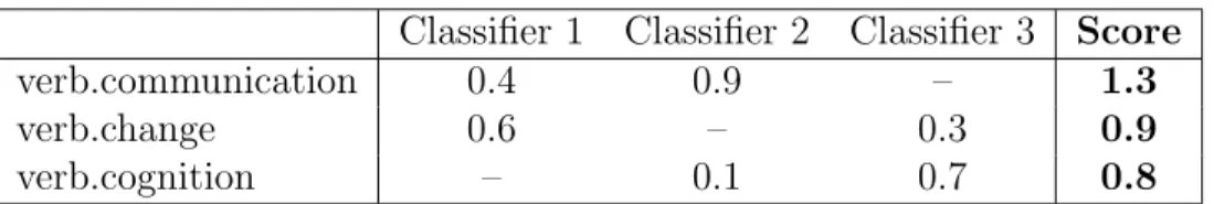
(29) Figure 3.16: Support Vector Machine separators trade-off between misclassification of training examples and the simplicity of the decision surface. Sklearn library can output the probability of each class when it is applied for the classification of unknown data or test data. The probability is used to choose one semantic class as the final output as will be explained in the next section.. 3.6. Selection of Semantic Class. The system chooses the only one semantic class for the given target word. The final step of the proposed method is to choose the most appropriate one from the results of several classifiers. A simple majority voting is introduced. Each classifier chooses one of two semantic classes. If the target word has two semantic classes and only one binary classifier is applied, the semantic class chosen by the classifier is the final output. When the target word has more than two semantic classes and two or more classifiers are applied, the semantic class that is most frequently selected by the classifiers is chosen as the final output. If two or more semantic classes are selected most frequently, a simple tie-break rule is applied. We choose the semantic class with the highest score, where the score is defined as the sum of the probabilities of the classification given by Sklearn library. Here is an example of how majority voting system works. Suppose that we have a target work “add” which belongs to three semantic classes: verb.communication, verb.change, and verb.cognition. Three classifiers are required: Classifier 1 selects either verb.communication or verb.change, Classifier 2 selects either verb.communication or verb.cognition, and Classifier 3 selects either verb.change and verb.cognition. Table 3.5 shows the probabilities of the semantic classes produced by three classifiers. In the example of Table 3.5, each semantic class is chosen once. Verb.communication is 21.

(30) Table 3.5: Example of Majority Voting verb.communication verb.change verb.cognition. Classifier 1 0.4 0.6 –. Classifier 2 Classifier 3 0.9 – – 0.3 0.1 0.7. Score 1.3 0.9 0.8. chosen by Classifier 2, verb.change is chosen by Classifier 1, and verb.cognition is chosen by Classifier 3. So the tie break rule is applied. The score of three semantic classes are shown in the last column in Table 3.5. Since the score is the highest, verb.communication is chosen as the final output.. 3.7. Feature Selection. Feature selection is a technique to automatically remove ineffective features to improve the performance of machine learning. It especially works well when the number of features is quite large, or the data samples are represented by high-dimensional feature vectors in other words. In this section, we present two methods for feature selection. One is a term-frequency based method, the other is Pearson’s Chi-squared Test.. 3.7.1. Frequency Based Feature Selection. Term-frequency is the number of times each term occurs in a corpus. Term-frequency based feature selection [23] is an effective method for reducing high-dimensional feature vectors in text classification. A term usually means a word in a text, but in this research, terms refer to the features in the training process. After counting the frequency of all terms (features), the method simply chooses the most frequent n features.. 3.7.2. Pearson’s chi-squared Test. Pearson’s chi-squared test (χ2 test) is a statistical test and is also a popular feature selection method that is widely applied for categorical data. This method evaluates the difference between the observed frequencies of the features and the expected frequencies under the null hypothesis H0 that assumes the feature and category (semantic class in this study) are independent. If the difference is large, then we can reject the null hypothesis H0 . It means that the feature is highly correlate with the category, implying the feature is effective for classification. In chi-squared test, the contingency table of the feature and category is constructed. In this research, the table of the feature and semantic class is built as shown in Table 3.6. In Table 3.6, O11 is the number of the data where the feature f appears in the context of the semantic class SC, O12 is the number of the data where the feature f appears in 22.

(31) Table 3.6: Contingency Table of Feature and Semantic Class SC 6= SC f. O11. O12. 6= f. O21. O22. the context of the other semantic classes, O21 is the number of the data where the feature f does not appear in the context of the semantic class SC, and O22 is the number of the data where the feature f does not appear in the context of the other semantic classes. Then, χ2 value is calculated from statistical data in Table 3.6 as Equation (3.1): N (O11 O12 − O12 O21 )2 χ = (O11 + O12 )(O11 + O21 )(O12 + O22 )(O21 + O22 ) 2. (3.1). where N is the total number of the data, or N = O11 + O12 + O21 + O22 . For all extracted features, χ2 values are calculated. Then the top n features with the highest χ2 value are selected.. 23.

(32) Chapter 4 Evaluation In this chapter, we describe an experiment to evaluate our proposed method. First, the experimental setup including the preparation of the test and training data will be explained. Then, the results of the experiments will be reported and discussed.. 4.1. Test Data. For the test data of the experiments, we used the training data of Senseval-3 English lexical sample task [16]1 . It is a collection of the sense tagged text for 57 target words. This data set contains only nouns, verbs, and adjectives as the target words. For each instance of the target word, the gold sense was mapped to the semantic class (the unique beginners in WordNet). However, only nouns and verbs were ambiguous in the semantic class level. Due to heavy computational costs for training SVM from a large data, it was difficult to conduct experiments for too many target words. Therefore, the nouns were not used in the experiment, either. In sum, the proposed method was evaluated for semantic class disambiguation of only verbs. However, this method can be applicable for any parts-of-speech. 1. Although both test and training data in this task were available, we chose the training data since it is larger than the test data.. 24.

(33) <instance id=“difference.n.bnc.00044017” docsrc=“BNC”> <answer instance=“difference.n.bnc.00044017” senseid=“difference%1:07:00::”> <answer instance=“difference.n.bnc.00044017” senseid=“difference%1:11:00::”> <context> Thoughts will be referred to as cognisant acts. The simplest and most fundamental aspect of cognisance ( fundamental philosophically and developmentally ) is what is usually referred to as self - world dualism : the knowledge that there is a physical world out there of which I am an experiencer and that is distinct from me . Mental development , on the constructivist view , consists in the elaboration of this knowledge ; so that if there is one central <head>difference<head> between the mental processes of the baby , the child , and of the adult it is in terms of how self - world dualism is manifest in ( and to ) the subject . The representational theory of mind treats the explanation of mental life as a kind of engineering problem ; it starts from the inside , from the representational state , and asks how mental states interact with one another to produce something that we would call knowledge ; the representational theorist proceeds like a sceptical philosopher who thinks that what figures in our mental life is not reality but our mental representations of it (recall my saying the Fodor described his position as methodological solipsism ) . The constructivist starting - point could not be more different , and might be said to be biological where the representational theory is engineering or machinological . </context> </instance> Figure 4.1: An Sample of Target Word ‘difference’ in Test Data We will show several examples of the instances in Senseval-3 data and explain how to prepare the test data in detail. Figure 4.12 and 4.2 show the examples of the instances of the target noun ‘difference’ and verb ‘begin’, respectively. In these figures, hinstancei marks up an target instance, hansweri marks up a gold sense, hcontexti marks up a context of a target instance and hheadi marks up a target instance itself. The ID of the target instance is represented in ‘id’ attribute of the hinstancei tag or ‘instance’ attribute of the hansweri tag. The character ‘n’, ‘v’ or ‘a’ after the first period is an abbreviation for noun, verb or adjective. In most cases, the hansweri tag appears once in a target instance as in Figure 4.2, but in some cases there are two or more hansweri tags as in Figure 4.1. It means that there are two or more gold senses per target instance. The annotators were allowed to assign multiple senses if they thought the target instance has two or more appropriate senses. 2. Although the nouns were not used as the target word, we have completed preparation of the experiment for the nouns such as extraction of the monosemous words, construction of the feature vectors and so on. Therefore, we show the example of the noun here.. 25.

(34) <instance id=“begin.v.bnc.00008477” docsrc=“BNC”> <answer instance=“begin.v.bnc.00008477” senseid=“369202”> <context> They are thus not simply a mentality derived from popular religion but from a traditional Roman catholicism which held sway in catholic Europe from the post - Reformation period and remained unchallenged until the 1960s . As will be seen in Chapter 5 , understanding this religious social consciousness requires some grasp of the traditional catholic teaching on the natural order and the good society , and how the nation is to respect the divine order established by God. An example of this can be taken from the recent contraception controversy in the Republic , which <head>began<head> in the 1960s . At that time , the Roman catholic archbishop of Dublin intervened in a pastoral letter in the following revealing terms : If they who are elected to legislate for our society should unfortunately decide to pass a disastrous measure of legislation that will allow the public promotion of contraception and an access hitherto unlawful to the means of contraception , they ought to know clearly the meaning of their action , when it is judged by the norms of objective morality and the certain consequences of such a law </context> </instance> Figure 4.2: An Sample of Target Word ‘begin’ in Test Data The gold sense is marked up at ‘senseid’ attribute in hansweri tag. The different sense IDs are used for nouns and verbs. The sense ID of the noun such as ‘difference%1:07:00’ or ‘difference:%1:11:00’ stands for an ID of WordNet synset. The list of the senses of the word ‘difference’ in WordNet are shown in Table 4.1. The table shows the sense ID, its corresponding synset and gloss in WordNet. The WordNet synset ID can be formatted as ‘WORD:%X:Y:Z’, where two digit number ‘Y’ stands for the semantic class ID shown in Table 3.1. Thus the sense can be easily mapped to its corresponding semantic class. On the other hand, the sense ID of the verb is not WordNet synset ID. It is represented as 6-digit numbers like ‘369202’ in Figure 4.2. In the Senseval-3 data, there is a table that defines the correspondence between the sense ID in Senseval-3 data and WordNet synset ID, as shown in Table 4.2. Using this table, the sense of the verb can be easily mapped to the WordNet synset ID and also its semantic class. The target instance was removed from the test data if two or more gold senses were assinged for it and these senses were mapped to the different semantic classes. Because our proposed system is designed to choose only one semantic class for one target instance. For example, in Figure 4.1, since two senses were mapped to the semantic class 07 (noun.attribute) and 11 (noun.event), this instance was discarded. Although there were 57 target words in Senseval-3 data set, not all of them were used in our experiment. As explained earlier, the adjectives and nouns were removed from the target word. Furthermore, if all instances of the target word has only one semantic class, it was not used for the evaluation. Because such target words were unambiguous in the semantic class level. In this way, 17 verbs remained as the target word in the experiment. 26.

(35) Table 4.1: Lexical Entry of the Noun ‘different’ sense ID difference%1:07:00::. difference%1:10:00::. difference%1:11:00::. difference%1:23:00::. difference%1:24:00::. synset difference. gloss (the quality of being unlike or dissimilar: ”there are many differences between jazz and rock”) dispute, difference, (a disagreement or argument about difference of opinion, something important; “he had a disconflict pute with his wife”; “there were irreconcilable differences”; “the familiar conflict between Republicans and Democrats”) deviation, diver- (a variation that deviates from the gence, departure, standard or norm; “the deviation from difference the mean”) remainder, differ- (the number that remains after subence traction; the number that when added to the subtrahend gives the minuend) difference (a significant change; “the difference in her is amazing”; “his support made a real difference”). Table 4.2: Lexical Entry of the Verb ‘begin’ sense ID 369201. synset ID begin%2:30:00::. 369202. begin%2:42:00::. 369203. begin%2:30:01::. 369204. begin%2:30:01::. synset begin, commence, set about, start begin, commence, originate, start begin, commence, kick off, lead, open, set about, start begin, inaugurate, initiate, start, undertake. gloss to perform the first step in a process; start. to come into being. to perform the first step of (something); start. to cause to come into being.. The table 4.3 shows a list of the target word as well as its potential semantic classes and number of samples in test data.. 27.

(36) Target. 4.2. Table 4.3: List of Target Word Semantic Classes. Test. activate. change, creation. 170. add. communication, change, cognition. 181. ask. communication, stative. eat. change, consumption. begin. change, stative. 68. climb. change, motion. 112. lose. competition, emotion, possession. treat. body, change, cognition, communication, social. 107. receive. communication, perception, possession. 48. encounter. competition, stative. 61. hear. cognition, perception, social. 24. remain. change, stative. rule. communication, social, stative. suspend. change, contact, social. watch. perception, social. 92. win. competition, possession. 42. write. communication, creation. 30. 95 144. 36. 135 57 116. Training Data. In this section, we present how we prepared training data for our proposed method. In this experiment, we only used monosemous words as the training data. Monosemous words are words which have only one semantic class in WordNet. Let us review the advantages and disadvantages to use monosemous words as the training data. The advantage of it is that we can use a raw text as the training data. Since the unique semantic class of the monosemous word can be regarded as the gold semantic class, no manual annotation is required for preparing labeled data. Therefore, it is easy to prepare a large amount of training data. The disadvantage is that the different words are used as the training samples of a certain semantic class. For example, as the samples of the semantic class ‘noun.act’, any words that have noun.act as its unique semantic class, such as ‘diet’ and ‘public’ , are used. However, the effective features for semantic class disambiguation may be different for different words. In other words, the features intrinsic to the words are lost in the monosemous word data. Anyway, we utilized a collection of monosemous words as 28.

(37) the training data. The Daily Yomiuri corpus [5] is used to construct the training data. It is a collection of English newspaper articles published in 2003. In the preparation process, all of monosemous words were extracted to separated files corresponding to one semantic class. In the files, each line represents a list of features extracted from a context of one target instance. We conducted two different experiments to evaluate our proposed method, which will be described in the following two subsections in details.. 4.2.1. Experiment I. Since it takes too long time to train the classifiers, we adopted the following three procedures to reduce the computational cost in this experiment. The number of the training samples were reduced to 10,000 per semantic class. These training samples were randomly chosen. Therefore, 10,000 × 2 = 20,000 training samples were used to train the classifier for one pair of the semantic classes. Table 4.4 shows the statistics of the training data in Experiment I. The column ‘SC’ indicates the number of potential semantic classes of the target word. In OVR-SCD, each one-versus-rest classifier is trained from 10,000 × 15 = 15,000 samples, since there are 15 semantic classes of the verb. The total number of the training sample shown in Table 4.4 is 15,000 multiplied by the number of classifiers or potential semantic classes. In PW-SCD, each pair-wise classifier is trained from 20,000 samples as denoted above. The number of the pair-wise classifiers is equal to the number of pairs of the potential semantic classes. If SC are 2, 3 and 5, 2 C2 = 2, 3 C2 = 3 and 5 C2 = 10 are the number of classifiers, respectively. The total number of the training samples shown in Table 4.4 is 20,000 multiplied by the number of the classifiers.. 29.

(38) Table 4.4: Statistics of Training Data in Experiment I Target SC OVR-SCD PW-SCD activate. 2. 300,000. 20,000. add. 3. 450,000. 60,000. ask. 2. 300,000. 20,000. eat. 2. 300,000. 20,000. begin. 2. 300,000. 20,000. climb. 2. 300,000. 20,000. lose. 3. 450,000. 60,000. treat. 5. 750,000. 200,000. receive. 3. 450,000. 60,000. encounter. 2. 300,000. 20,000. hear. 3. 450,000. 60,000. remain. 2. 300,000. 20,000. rule. 3. 450,000. 60,000. suspend. 3. 450,000. 60,000. watch. 2. 300,000. 20,000. win. 2. 300,000. 20,000. write. 2. 300,000. 20,000. Second, since the dimension of the feature vector was huge, the number of the features was limited. Frequency based feature selection, which was explained in Subsection 3.7.1, was applied. That is, the n most frequent features were selected, where n stands for the number of the features. We evaluated the baseline (Ariyakornwijit’s method) and our method with n = 5000, n = 7, 000 and n = 10, 000 in a preliminary experiment. Since the case of n = 7, 000 was the best, we will show the results of the methods with 7,000 features in the Section 4.3. Finally, since Sklearn library can control the maximum number of iteration in the training of SVM, we limit the iteration times. At first, SVM classifiers were trained by the maximum of 1,000 iteration, and the performance of the baseline and our method was compared. Then, for only our method, the classifiers were trained with an unlimited number of iteration to improve the performance. In this case, the iterative learning of SVM was continued until it converged.. 4.2.2. Experiment II. In Experiment I, the number of the training samples per semantic class was fixed. However, such a setting is inappropriate to evaluate the proposed method. The motivation 30.

(39) of our method is to correct the imbalance of the positive and negative samples. In the training data constructed in Experiment I, the ratio of the positive and negative samples was not naturally but artificially determined. Therefore, we reconsidered the way how to reduce the computational costs. Experiment II was carried out as follows. First, the size of the Daily Yomiuri corpus was reduced to 20,000 lines, where each line roughly corresponded to each sentence. The first 20,000 lines in the file of Daily Yomiuri were simply extracted to construct a reduced sized corpus. Then, the monosemous words were extracted as the training samples from it. Although the size was decreased, the distribution of the semantic classes in the whole corpus might be kept in the reduced sized corpus. The Table 4.5 shows the statistics of the training data in experiment II. Table 4.5: Statistics of Training Data in Experiment II Target SC OVR-SCD PW-SCD activate. 2. 531,346. 16,366. add. 3. 797,019. 29,219. ask. 2. 531,346. 53,483. eat. 2. 531,346. 19,512. begin. 2. 531,346. 55,131. climb. 2. 531,346. 12,822. lose. 3. 797,019. 74,168. treat. 5. 1,328,365. 70,010. receive. 3. 797,019. 68,147. encounter. 2. 531,346. 59,812. hear. 3. 797,019. 78,705. remain. 2. 531,346. 55,131. rule. 3. 797,019. 97,979. suspend. 3. 797,019. 30,715. watch. 2. 531,346. 69,721. win. 2. 531,346. 49,260. write. 2. 531,346. 14,718. Next, the dimension of feature vector was limited to 7, 000. For feature selection, Pearson’s chi-squared test based feature selection presented in Subsection 3.7.2 was applied. Finally, the maximum number of iteration controlled by Sklearn library was increased to 5,000 iterations. Comparing to Experiment I, this experiment took more computational cost and time since the dimension of feature vector was the same but the training data and the maximum number of iterations was larger.. 31.

(40) 4.3. Results. An evaluation criterion is accuracy of prediction of the semantic classes. This is a traditional measurement widely used in most of the classification tasks. It is measured by the ratio of the number of correctly predicted instances to the total number of target instances.. Accuracy =. Number of correctly classified samples Total number of test samples. (4.1). A baseline system is the Ariyakornwijit’s method (OVR-SCD) [1]. Their system originally chooses two or more semantic classes for each target instance. On the other hand, our system always chooses only one semantic class. To compare the baseline and our system, Ariyakornwijit’s method is revised to select one semantic class per instance in our implementation. If two or more classifiers judge as ‘yes’, the semantic class of the highest probability provided by Sklearn library is chosen. Since this revision is required for comparison with our system, we implemented Ariyakornwijit’s method as the baseline by ourselves.. 4.3.1. Results of Experiment I. Table 4.6 reveals the accuracy of the baseline (OVR-SCD) and our method (PW-SCD) with the maximum 1,000 iteration training, and our method with no limit of iteration times (PW-SCD+ ). The last row indicates the micro average of the accuracy for 17 target words. The overall performance of our proposed pair-wise semantic class disambiguation was better than the previous one-versus-rest approach. The micro average of PW-SCD was improved by 1.4 % comparing with OVR-SCD. The accuracy was quite high for several target words, for example, 87% for the target word ‘write’. For the other several words, however, the accuracy was low, e.g. 0.7% for ‘eat’and 2.7% for ‘climb’. PW-SCD always chose the semantic class “change” for these two target words, but there were only 1 and 3 instances of “change” in the test data of ‘eat’ and ‘climb’, respectively. It might be caused by the limitation of training iteration, since the accuracy of PW-SCD+ was much improved. Furthermore, the improvement by our method also highly depended on the target word. For the target word ‘begin’, ‘receive’, ‘encounter’, ‘suspend’, ‘watch’, and ‘write’, PW-SCD remarkably outperformed OVR-SCD by 15-65%. On the other hand, the accuracy greatly decreased for ‘ask’, ‘eat’, ‘remain’, and ‘rule’. These results indicate that the appropriate architecture of the semantic class disambiguation, one-versus-rest or pair-wise, might be different for the target word. If we could guess more appropriate method for the target word and apply it for disambiguation, the overall performance would be improved much. Investigation of this direction is our important future work. Let us compare PW-SCD and PW-SCD+ . When the number of iteration in SVM training was unlimited, the micro average was improved by 10% and reached around 50%. 32.