JAIST Repository https://dspace.jaist.ac.jp/

(1)

Japan Advanced Institute of Science and Technology

JAIST Repository

https://dspace.jaist.ac.jp/

Title 多変量経験的モード分解を利用した音源フィルタモデ

ルに基づく音声分析法

Author(s) Surasak, Boonkla Citation

Issue Date 2018‑03

Type Thesis or Dissertation Text version ETD

URL http://hdl.handle.net/10119/15326 Rights

Description Supervisor:鵜木祐史, 情報科学研究科, 博士

(2)

Speech Analysis Method Based on Source-Filter Model Using Multivariate Empirical Mode

Decomposition

by

Surasak BOONKLA

submitted to

Japan Advanced Institute of Science and Technology in partial fulfillment of the requirements

for the degree of Doctor of Philosophy

Supervisor: Professor Masashi Unoki

School of Information Science

Japan Advanced Institute of Science and Technology

March, 2018

(3)

(4)

Abstract

The growth of speech processing technology within the last few decades enables us to communicate with each other even when we are too far apart by using speech. It is not only human-to-human but also human-to-machine communication that become important and play a vital role in our daily life. However, the speech communication is always damaged by environmental noises. Moreover, multiple echoes (reverberation) within a confined space cause severe reduction of speech intelligibility as well. These drawbacks exist since the beginning of the speech communication. To date, researchers are attempting to solve these problems because they still degrade the communication systems.

Since the availability of digital hardware, there has been much research in speech processing technology especially speech analysis which is the backbone of several applications such as voice activity detection, speech enhancement, automatic speech recognition, speaker recognition, and hearing aids. The performance of these applications degrades drastically in real environments because the speech analysis method employed by these applications is not robust against noises and reverberation. We aim to propose the robust speech analysis method by using multivariate empirical mode decomposition (MEMD).

The motivation of using MEMD is that it can extract the oscillation components and make the signal sparse by reducing the degree of mixing. This ability can reduce the degree of mixing of noises in the noisy speech signals. Furthermore, MEMD can automatically separate the signals which are resulted from the addition of sub-signals. For example, automatic source-filter separation, automatic noise separation, and automatic separation of cepstrum of room impulse response. Therefore, the MEMD-based speech analysis method can ideally be able to fulfill the following requirements. (i) the source and vocal tract information are obtained simultaneously. (ii) robust against noise. (iii) robust against reverberation, and (iv) robust against both noise and reverberation.

This research aims to solve the problems of speech analysis in real environments by proposing the robust MEMD-based speech analysis method. It exploits specific properties of MEMD as follows: (1) it can analyze the non-stationary signal. Since speech signal is the non-stationary signal, MEMD should be the appropriate approach for speech analysis.

(2) It is the nonparametric and data-driven approach. MEMD does not impose any assumption regarding the input signal. (3) It can automatically separate mixtures of signals or reduce the degree of mixing. (4) It can automatically align the common component into the same index of sub signal namely intrinsic mode function (IMF). However, the challenge of using MEMD is how to correctly categorize IMFs derived from MEMD into groups of sources, vocal tract, noise, reverberation. Four main tasks would be focused on to achieve the final goal of this research. That is MEMD-based speech analysis method in (a) clean, (b) reverberant, (c) noisy, and (d) noisy reverberant environments. Then the proposed speech analysis method will be applied to some practical applications to show its effectiveness.

If estimates of speech features can be further improved by the proposed method in real environments, it would directly have a great impact on the society of speech signal processing. It would also contribute to the engineering and technology in the sense that

(5)

the performance of several critical applications, for example, voice activity detection, speech recognition, hearing aids, speech enhancement, and communication systems would be enhanced. Furthermore, it would have the indirect contribution to human society when the performance of such applications is improved. Throughout this dissertation, the reader will see how our proposed speech analysis is carried out in clean, noisy, and reverberant conditions. Some applications, based on the techniques used in our speech analysis, such as voice activity detection, noise reduction, and speech dereverberation are demonstrated as well. We proposed MEMD-based speech analysis for clean speech that is superior to linear prediction and cepstrum based methods in F₀ estimation. In noisy conditions, we cooperated the MEMD-based noise reduction technique with the MEMD-based speech analysis method so that the speech analysis could be robust. In reverberant conditions, we could reduce the effects of reverberation by using MEMD so that the speech analysis could be robust. The final goal of speech analysis in noisy reverberant conditions have not yet completed and will be our future work.

Keywords: speech analysis, source-filter model, multivariate empirical mode decomposition, noise reduction, dereverberation

(6)

Acknowledgments

This research started from my interest in speech signal processing, especially in reverberant environments. The important person who provided the research seed to me is Professor Masashi Unoki. I sincerely appreciate the time he spent teaching me. His constantly energetic research activities and encouragement helped me a lot in my Ph.D.

course. I appreciate his broad and profound knowledge and patience on me. It seems to be no good solution in this research without his supervision. Professor Masato Akagi is another important person. I also sincerely appreciate his useful questions and comments which helped me improve my knowledge and skills when I presented in laboratory meetings and rehearsals. I would like to thanks to Professor Stanislav S. Makhanov of Sirinthorn International Institute of Technology who always encourages and helps me a lot. His useful suggestions help me manage several difficulties in my Ph.D. life. My Boss, Professor Dr. Chai Wutiwiwatchai, is another important person. I appreciate his patience, useful suggestions, and comments. I appreciate the support from Dr.Kwan Sitathani, the former director at NECTEC, Dr. Thanaruk Theeramunkong and Associate Professor Dr.

Waree Kongprawechnon of Sirinthorn International Institute of Technology who gave me the chance to join this SIIT-JAIST-NECTEC dual degree program. Without them, I might not have studied in this program. Furthermore, I greatly appreciate the grants in JAIST research grant and A3 Foresight program that support the budget for joining the conferences. I am also grateful to all my teachers who taught, suggested me, my parents who always stand by my side.

Lastly, I would like to express my thanks to the Buddha Gotama for having taught several precepts that guide me throughout my life. Without his precepts, I could not imagine what kind of life I would be. I would like to attribute my goodness to him as well as noble monks and all of the devas who taught and inspired me to do good things.

(7)

List of Figures

1.1 Speech analysis/synthesis . . . 3

2.1 Speech production model . . . 7

2.2 Speech production methanism and airflow in the glottis . . . 8

2.3 Spectral shaping . . . 10

2.4 Demostration of speech analysis using LP . . . 12

2.5 Demostration of speech analysis using CEP . . . 13

2.6 Demonstration of sifting process . . . 17

2.7 Demonstration of bivariate EMD . . . 18

2.8 Example extrema of bivariate signal at a given instant in time . . . 19

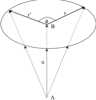
2.9 Rotation of a vector r around a unit vector u or line segment AB by and angle φ. . . 20

2.10 Illustration of common mode alignment [27] . . . 22

2.11 EMD as filter banks [27] . . . 22

3.1 Block diagram of MEMD-based speech analysis . . . 25

3.2 Log magnitude spectrum and their IMFs. The autocorrelation of IMFs are the red lines. Summation of the IMFs order from 1 to 4 shows the periodic feature of harmonicx of the souce as illustrated in the last row. . . 28

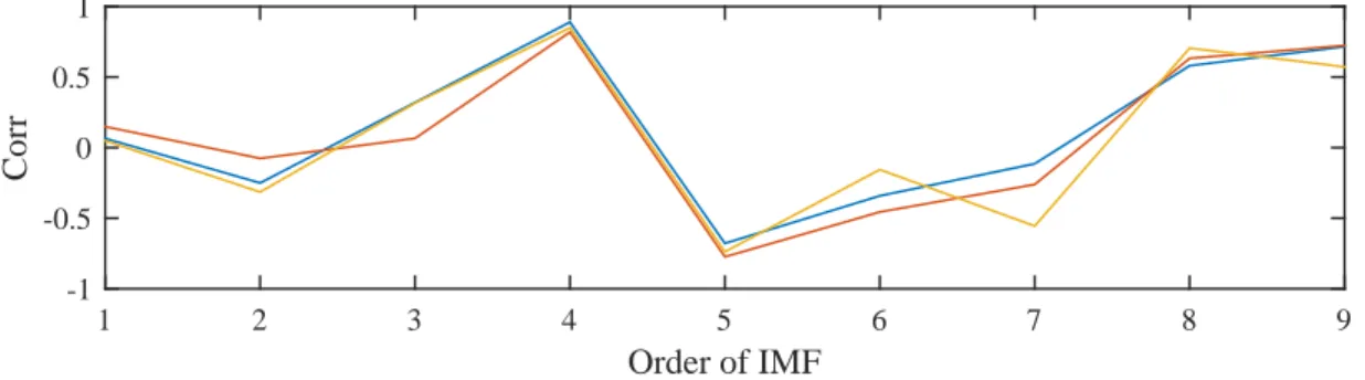
3.3 Correlation coefficient between IMFs. The three lines are from three different pairs (columns) of IMFs. . . 29

3.4 F0 estimation of synthesized voices . . . 30

3.5 Estimated F₀: (a) a speech signal, (b) estimatedF₀ from LP-based (blue), CEP-based (red), and proposed (orange) methods. . . 30

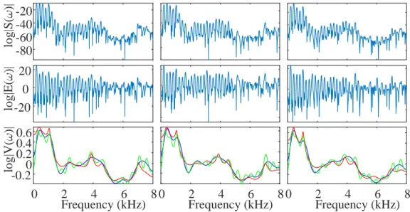
3.6 Source-filter sepration. The top panels show log|S(ω)| from three frames. The middle panels show log|U(ω)|, and the bottom panels show log|V(ω)| compared with spectral envelopes obtained by LP and cepstrum are plotted bottom panels. . . 31

3.7 The results of formant estimations of (a) synthesized and (b) spoken voices 37 4.1 Log magnitude spectra [log|S(ω)|], their IMFs [c_k(ω)], and autocorrelation of IMFs (red lines). . . 41

4.2 Source-filter separation and estimated F₀. (a) Log magnitude spectrum, (b) fine structure, (c) spectral envelope, (d) clean speech signal, (e) noisy speech signal, and (f) estimated F0. . . 42

4.3 Spectral envelopes and their peaks . . . 43

4.4 Block diagram of the speech analysis framework in noisy conditions . . . . 44

4.5 Input signals (first row), IMFs of input signals (ck), and power envelopes of IMFs (red). . . 45

(10)

4.6 Euclidean distance, signals, and estimated F0: (d) – (e) estimated F0 of (a) is the blue line and those red lines are of (b) and (c). (f) blue, red, and

orange lines associate with three pairs of column of IMFs in Fig. 4.5. . . . 46

4.7 VAD using estimatedF0 . . . 47

4.8 Spectral envelopes . . . 48

4.9 Results ofF₀ estimation: MEMD denotes the MEMD-based speech analysis. IMCRA is the estimatedF0 after noise reduction by using IMCRA [49]. 50 4.10 Formant estimation of vowel /AH/: the ground-truth are circles. Before noise reduction are the red diamonds (noisy), green stars (CEP), and black squares (LP). After noise reduction are IMCRA blue triangles (IMCRA), and the red crosses (proposed). . . 51

4.11 Formant estimation of vowel /IY/: the ground-truth are circles. Before noise reduction are the red diamonds (noisy), green stars (CEP), and black squares (LP). After noise reduction are IMCRA blue triangles (IMCRA), and the red crosses (proposed). . . 51

4.12 Formant estimation of vowel /UW/: the ground-truth are circles. Before noise reduction are the red diamonds (noisy), green stars (CEP), and black squares (LP). After noise reduction are IMCRA blue triangles (IMCRA), and the red crosses (proposed). . . 52

4.13 Formant estimation of vowel /EY/: the ground-truth are circles. Before noise reduction are the red diamonds (noisy), green stars (CEP), and black squares (LP). After noise reduction are IMCRA blue triangles (IMCRA), and the red crosses (proposed). . . 52

4.14 Formant estimation of vowel /OW/: the ground-truth are circles. Before noise reduction are the red diamonds (noisy), green stars (CEP), and black squares (LP). After noise reduction are IMCRA blue triangles (IMCRA), and the red crosses (proposed). . . 53

4.15 Evaluation of spectral envelope from all kind of noises . . . 53

5.1 Reflections of speech signal in an enclosed space . . . 56

5.2 A room impulse response . . . 56

5.3 Source and filter in quefrency domain . . . 58

5.4 Reverberation as additive noise . . . 59

5.5 Estimated formants from clean, reverberant, and enhanced speech signals . 60 5.6 Ensemble average complex cepstrum . . . 61

5.7 Average cepstrum of (a) clean speech (blue line, ensemble average), [(b) and (d)] room impulse response, [(c), (f), and (g)] reverberant speech (ensemble average), and (e) estimated cepstrum of RIR . . . 62

5.8 IMFs of average minimum-phase amplitude cepstra . . . 64

5.9 Similarity measurement between IMFs at the IMF order . . . 65

5.10 Estimated minimum-phase amplitude cepstrum of RIR, where MPC denotes minimum-phase cepstrum. Panel (a) is the first estimate of MPC of RIR. Panel (b) is the estimate of MPC of clean speech. Panel (d) is the second estimate of RIR MPC by using the estimate of MPC of clean speech in a high quefrency range. Panel (e) is the true RIR MPC. . . 67

5.11 Demonstration of the dereverberated speech signal based on minimum- phase cepstrum enhancement. . . 68

(11)

5.12 Spectrogram of the dereverberated speech signals, where MP and APP

mean minimum-phase and all-pass phase enhancement. . . 69

5.13 Energy distribution of all-pass phase cepstrum . . . 70

5.14 Block diagram of speech analysis in reverberant environments . . . 71

5.15 Correct rate of F₀ estimation base on error margin = 10% . . . 72

5.16 Estimated formants of /AH/ from clean (black circles), CEP-Based method (red triangles), LP-based method (blue squares), and the proposed framework (black crosses). . . 72

5.17 Estimated formants of /IY/ from clean (black circles), CEP-Based method (red triangles), LP-based method (blue squares), and the proposed framework (black crosses). . . 73

5.18 Estimated formants of /UW/ from clean (black circles), CEP-Based method (red triangles), LP-based method (blue squares), and the proposed framework (black crosses). . . 73

5.19 Estimated formants of /EY/ from clean (black circles), CEP-Based method (red triangles), LP-based method (blue squares), and the proposed framework (black crosses). . . 74

5.20 Estimated formants of /OW/ from clean (black circles), CEP-Based method (red triangles), LP-based method (blue squares), and the proposed framework (black crosses). . . 74

6.1 Demonstration of robust feature for VAD where the proability of speech present is shown in the last row. . . 76

6.2 Demonstration of VAD using estimated F0 . . . 77

6.3 Results of VAD . . . 78

6.4 Results noise reduction . . . 79

6.5 Block diagram of the proposed denoise and evaluation framework . . . 80

6.6 Objective evaluation of speech quality . . . 82

6.7 Objective speech intelligibility evaluation by using ABC-MRT16 [82] . . . . 82

6.8 Results of listening test . . . 83

(12)

List of Tables

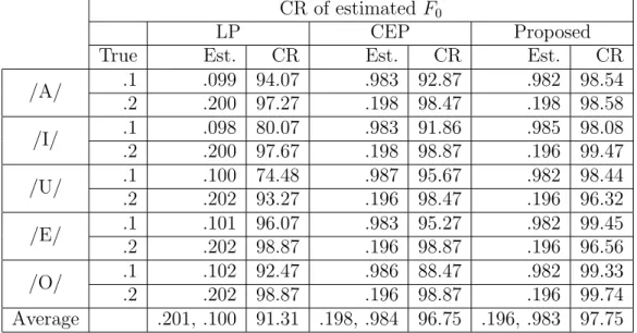
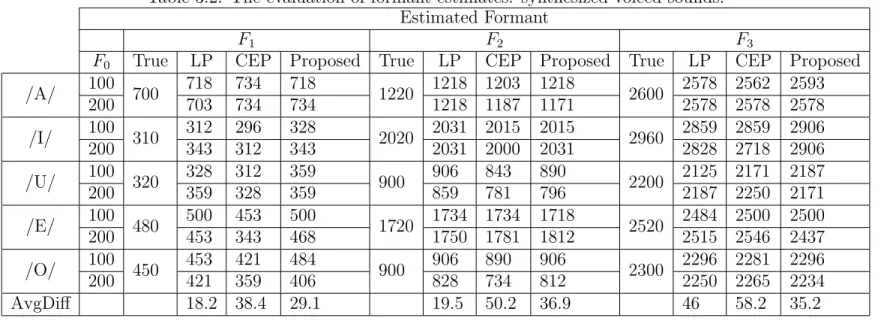
3.1 The correct rate (CR) of F₀ estimates of the synthesized voiced sounds where the unit of the true (True) and estimated (Est.) values are kHz. . . 33 3.2 The evaluation of formant estimates: synthesized voiced sounds. . . 35 3.3 The results of formant and F₀ estimations of real voices. The standard

deviation (SD) of the estimated F₀ when CR=100% and formant was estimated is also shown. . . 35 3.4 Result of spectral envelope evaluation by using average and correlation

coefficient (CorCoef), Euclidean (EU), Itakura-Saito (IS), log spectral (LS) distances. The P, L, and C are the proposed, CEP-based, and LP-based methods, respectively. . . 36 5.1 Spectral envelope measurements, where Rvb and Enh denote reverberant

and enhanced speech. . . 71 6.1 PESQ evaluation of noisy and enhanced speech signals . . . 80

(13)

Notation

t independent variable in time domain ω independent variable in frequency domain t˜ independent variable in quefrency domain δ(t) delta function

F₀ pitch or fundamental frequency F_n the n-th formant frequency s(t) speech signal

g(t) glottal flow waveform

u(t) pulse train of glottal flow waveform v(t) vocal-tract impulse response

p(t) impulse train c(˜t) cepstrum

C(˜ˆ t) complex cepstrum

w(t, τ) window function centering at timeτ S(ω) Fourier transform of s(t)

U(ω) Fourier transform of u(t) V(ω) Fourier transform of v(t) G(ω) Fourier transform of g(t) P(ω) Fourier transform of p(t)

W(ω, τ) discrete-time Fourier transform ofw(t, τ) e[k] prediction error

E· mathematical expectation a_p the p-th prediction coefficient J(·) a cost function

q_k(t) the k-th intrinsic mode function in time or quefrency domain q_k(ω) the k-th intrinsic mode function in frequency domain

r(t) residue, monotonic signal or function e(t) envelope signals

m(t) average signal from envelope signals C(˜ˆ t) complex cepstrum

¯i,k,¯ ¯k unit vectors along x, y, and z axes o unit quaternion

u unit vector

r a vector

p^φ_θ(t) projection of a signal on a direction vector defined byφ and θ

< real part

= imaginary part

T60 reverberation time

(14)

Acronym and Abbreviation

EMD empirical mode decomposition BEMD bivariate EMD

CEMD complex EMD

TEMD trivariate EMD

RI-EMD rotation-invariant EMD MEMD multivariate EMD IMF intrinsic mode function RIR room impulse response FFT fast Fourier transform LSD log-spectral distance PSD power spectral density LP linear prediction

CEP ceptrum

ISD itakura-saito distance

DTFT discrete time Fourier transform

IDTFT inverse discrete time Fourier transform SVD singular value decomposition

IF instantaneous frequency MMSE minimum mean-square error SS spectral subtraction

WN Weiner filter src glottal source flt vocal tract

LSA log spectral amplitude estimator FRR false rejection rate

FAR false acceptance rate

PESQ perceptual evaluation of speech quality

IMCRA improved minima controlled recursive averaging

(15)

Chapter 1 Introduction

1.1 Overview and history of speech analysis

The nature of speech signal has been studied for more than thirty years. The speech signals from our mouth are similar to the sounds resulting from exciting the resonance cavities by the source signal from the vibrating reed. Changing the shape of the resonance cavities causes different sounds which are similar to changing the shape of the vocal tract in our throat. Based on this fact, in 1769 Kratzenstein invented the talking machine that can produce the voiced sounds of five vowels in 1769. In 1930, Dudley found that speech signal is the amplitude-modulated signal. That is the message which represents the thoughts of the speaker to be conveyed to the listener is imprinted on the quasi-periodic or noisy carrier signals. The message is the time-varying shape of the vocal tract, moving frequencies ranging from 0 to 20 Hz, that modulate the carrier signals passing through it.

Based on this understanding, Dudley invented several devices using two important principles: voder and vocoder. Voder is a flexible talking machine which is able to produce arbitrary sentences whereas vocoder is an attempt of compressing speech by keeping only the time-varying modulated amplitude. Since the modulating frequencies of the vocal tract are not over 20 Hz, he tried to send this message via a narrow bandwidth channel.

He also introduced the spectrograph which displays the time-frequency distribution of the energy of speech signal. His research inspired many researchers around the would so that a considerable amount of research regarding the various aspects and properties of speech signals. Since the availability of the digital hardware, the research in speech signal processing has much been developed, especially in speech coding for efficient communication, speech recognition, speech synthesis, and hearing aids.

Another aspect of the speech signal is that it is the continuously-varying air pressure propagating out from our mouth. It is induced into the continuously-varying electric voltage by a microphone. In digital hardware, this voltage is converted or sampled into a sequence of numbers, referred to as a discrete-time signal, by analog-to-digital (ADC) converter so that the speech signal can be digitally transmitted and processed. Digital speech signal processing can be defined as the manipulation of that sequence to obtain some properties of the signal relating to the carrier and the modulating vocal tract or a new signal with some desired properties. This process is normally known as the pair of speech analysis/synthesis.

The speech analysis process usually bases on a speech production model to obtain the desired properties of the speech signals. For example, consider a model of speech

(16)

production when the air passes from the lung through the vocal or nasal tract and go out from the lips. When air flows past the vocal cords, the vocal cords periodically vibrate the rate of which gives the pitch or fundamental frequency, F₀, of the voiced sounds. If we could measure the air pressure after the vocal cords, the waveform of the air pressure will be the periodic pulses which act as an excitation source to the cavity between the vocal cords and the lips or the nose namely, the vocal or nasal tract.

The vocal or nasal tract behaves like a resonator modifying the spectrum of the pulses train of the air pressure waveform. Based on this knowledge, the simple model namely the source-filter model can be built. The general assumption used in speech signal analysis/synthesis is that the vocal tract is the time-invariant system so that the output speech signal is said to be to the convolution of the pulse-train source with the impulse response of the vocal tract. Consequently, the variation of the excitation source and shape of the vocal tract results in a typical speech utterance which composes of a sequence of vowels and consonants the spectrum of which change with time.

After obtaining the desired properties of the speech signal, one can produce speech signal by speech synthesis by using the same or modified properties. The model of speech perception, on which we will not focus on this dissertation, of the receiver may be taken into consideration for modification of the speech properties. The objectives of modification may be (i) to enhance speech intelligibility such as speech enhancement and (ii) to hide some information that can not be perceived by the listener such as speech watermarking.

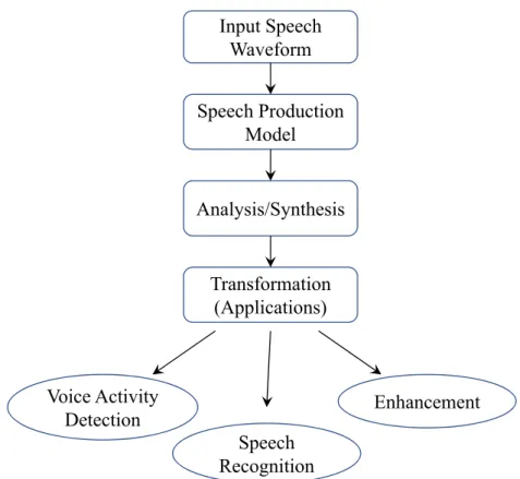
Therefore, speech analysis and speech synthesis is a pair of speech processing techniques that always come together as illustrated in Fig. 1.1.

Based on the speech production described above, the general speech analysis/synthesis systems can be signed as shown in Fig. 1.1 where the analysis process takes apart the speech waveform to extract the underlying parameters of the time-varying system of the vocal tract. The analysis is performed with the temporal and spectral resolution that is adequate to measurement such underlying parameters. In synthesis process, the waveform is put back based on the estimated or modified parameters and models. An objective of the block diagram in Fig. 1.1 is to design an identity system that the output equals the input when no speech parameters modification is performed. This diagram is the backbone for several applications that transform the speech waveform into some desirable form.

1.2 Speech analysis technigues: state-of-the-art

Since the availability of digital hardware, there are several proposed speech analysis methods most of which are based on the source-filter model. Classically, there are two techniques frequently employed in the speech analysis: cepstrum (CEP) and linear prediction (LP) [1]. Since vocal tract is the time-invariant system, the coefficients of vocal tract filter which is represented by an all-pole filter model are estimated by LP based on autocorrelation or covariance techniques [2]. The estimate of the source signal (e.g. periodic pulses) is obtained by inverse filtering the input speech signal. The inverse filter comes from the reciprocal of the all-pole filter. One disadvantage is that the all-pole filter model does not match some voiced sounds results from the speech model having zeros such as voiced fricatives and nasals. The stochastic model based autoregressive moving average model (ARMA) [3] handles this weak point of LP by estimating both zeros and poles with

(17)

Input Speech Waveform

Speech Production Model

Analysis/Synthesis

Transformation (Applications)

Voice Activity

Detection Enhancement

Speech Recognition

Figure 1.1: Speech analysis/synthesis the assumption of highly accurate speech production model.

CEP is the homomorphic transformation that inverse Fourier transforms log magnitude spectrum of the speech signal in frequency domain to cepstrum coefficients or cepstrum in quefrency (time) domains. The spectrum of voiced speech signal consists of the superposition of spectral fine structure and the spectral envelope correspondings to the source waveform output from the larynx and the frequency response of vocal tract.

Specifically, the voiced sound results in periodic feature of harmonics. Therefore, the cepstrum coefficients of the voiced sound are usually the peaks in the high quefrency range. The frequency response of the vocal tract is the spectral envelope the cepstrum coefficients of which lies in the lower range of the quefrency. The cepstrum coefficients of the source can be separated from the cepstrum coefficients of the vocal tract, or vice versa, by filtering in the quefrency domain or liftering [4].

To date, besides the methods mention above, there are several proposed speech analysis methods, for example analysis-by-synthesis (AbS) [5], STRAIGHT [6] [7] [8], and empirical mode decomposition (EMD) [9] – [23] based method. AbS is widely used in the source analysis, speech recognition systems, and speech coding algorithm. The term analysis- by-synthesis refers to an analysis process applied to the signals which are produced by the signal generator. The signal generator begins the signal synthesis process with some initialized properties. Thus, the heart of the AbS is the signal generator. The analysis and synthesis processes are carried out until the error between the input and synthesized signal reaches some smallest value, at which analyzer indicates the properties of the synthesized signal. The input signal is required to be clean to obtain the accurate properties of the input signal, which implies that AbS is not robust in real environments.

(18)

The heart of STRAIGHT is the convolution of the hamonicity of speech spectrum by the spectrum of the analysis window function. In other words, it uses the spectrum of a particular window function to interpolate the harmonic features of the speech spectrum by the summation of the main lobes of the window function [7] [8]. Therefore, the accurate F₀ estimation is required by STRAIGHT for the interpolation. Most of the EMD-based methods have been proposed so far have been utilized for F₀ in the time and frequency domain [10] – [23]. Besides the source analysis, we have also proposed the multivariate EMD for the vocal tract filter analysis [12] [13]. The main idea of EMD is that it can extract the oscillating components which are the periodicity of the speech signal in the time domain or the harmonicity of log spectrum of speech in the frequency domain by iterative sifting. Another advantage of using EMD is that it makes the input sparse by decomposing it into band-limited sub-signals namely intrinsic mode functions (IMFs) some of which are the desired signal.

According to the literature, by using a speech analysis method, the information of speech signal relating to the source waveform output from the larynx and the information of vocal tract can be obtained. On the basis of the source-filter model, the source waveform and the vocal-tract impulse response are usually separated so that the effects from the other is minimized. Some parameters are required by the above speech analysis methods such as the sampling rate dependent prediction order and the gender-dependent cut-off quefrency which are required by the LP and CEP-based speech analysis methods.

STRAIGHT requires the accurate F₀ estimation for the harmonic peaks interpolation.

Moreover, most of them are very weak against noises and reverberation in real environments. Some can be robust against noises to a certain extent but still underperform in practical applications. EMD has some properties, described later, that seems to be able to handle noises and reverberation. Therefore, we will use it to propose the robust speech analysis method in real environments.

1.3 Motivation and research goal

The motivation for this research came from the persistent to overcome the limitations of existing speech analysis methods when they are exploited in real environments. How to obtain the accurate speech parameters in very noisy reverberant environments is always in our mind. If these limitations can be overcome, it would have a great impact on the research society of speech signal processing.

According to the ability of EMD that can extract the oscillation component and make the signal sparse by reducing the degree of mixing, it is possible to propose a robust speech analysis by using EMD. In the case of clean speech, EMD can adaptively separate the source and filter and extract the periodicity or harmonicity. In noisy environments, additive background noises can become sparse when noisy speech signals are decomposed into IMFs, and some noise can be mostly separated from the target speech signals. In reverberant environments, the room impulse response can be separated from the target signal when the reverberant speech signals are converted into cepstrum. Therefore, the robust speech analysis method in real environments can be archived by combining the concepts described above.

The final goal of this research is to solve the problems of speech analysis in real environments. Some subgoals are set in this dissertation to reach the final goal. That is

(19)

1. Speech analysis of clean speech signal using multivariate empirical mode decomposition

2. Robust speech analysis based on empirical mode decomposition in noisy environments

3. Robust speech analysis based on empirical mode decomposition reverberant environments

4. And finally, robust speech analysis method based on empirical mode decomposition in noisy reverberant environments

In the end, some applications will be demonstrated to show the effectiveness of the proposed speech analysis method.

1.4 Thesis outline

There are seven chaters in this dissertation. The remainder are organized as follows.

Chapter 2 mentions about the necessary background knowledge such as the source- filter model, classical speech analysis methods such as LP and CEP. Since the proposed speech analysis method is based on EMD, EMD and its extensions including their advantages and disadvantages are described in this chapter.

Chapter 3 explains the important concepts used in the proposed speech analysis method based on multivariate empirical mode decomposition. We start with the simplest one, clean speech analysis, in comparison with the LP and CEP-based methods. The re- markable advantages are emphasized. Also, the general evaluation measures are described for evaluating the proposed speech analysis.

Chapter 4 demonstrates the first extension of the proposed speech analysis method in noisy conditions. There are two stages which are noise analysis/reduction and speech analysis. The first stage emphasizes the advantage of EMD in noise reduction compared with other methods. The second stage is the proposed method of Chapter 3.

Chapter 5demonstrates the second extension of the proposed speech analysis method in reverberant conditions. There are also two stages which are dereverberation and speech analysis. The complex cepstrum cooperates with the EMD for dereverberation in the first stage. The proposed speech analysis described in Chapter 3 is in the second stage.

Chapter 6 gives examples of applications of the proposed speech analysis method:

voice activity detection (VAD), denoising, and dereverberation. The VAD is achieved by using speech analysis. This VAD is further applied to the second application, denoising, the results of which are compared with the well-known method. The third application is speech dereverberation which enhance reverberant speech signals by using complex cepstrum. PESQ is used for evaluation of denoising and dereverberation.

Chapter 7 addresses the summary of this work and its contributions to this research fields. Since there are still limitations, we will discuss about the future improvement.

1.5 Summary

The innovative and unique points of our speech analysis method can be sum up as follows:

(1) this research exploits the advantages of MEMD for speech analysis which can estimate

(20)

both source and filter information, (2) it can adaptively separate the source and the vocal tract filter, noise and speech, reverberation and speech. In short, we began this chapter by providing answers to the questions: what is the problem to be solved? why we have to solve? and is it challenging to solve?. After that, the motivation and goal of this research were described. The structure of this dissertation was lastly outlined.

(21)

Chapter 2 Background

2.1 Speech production: source-filter model

Basically, speech signals come from the air passes from the lung through the vocal or nasal tract and go out from the lips. When air flows past the vocal cords, the vocal cords periodically vibrate the rate of which gives the pitch or fundamental frequency, F₀, of the voiced sounds. The periodic pulses of air after the vibration behave like an excitation source flowing into the cavity between the vocal cords and the lips or nose namely vocal or nasal tract. The vocal or nasal tract behaves like a resonator that modifies the spectrum of the periodic air flow. Based on this fundamental knowledge, a simple speech production model namely the source-filter model has been constructed. The vocal tract is usually assumed to be the time-invariant system so that the air pressure output from the lips is the convolution of the periodic air pressure waveform after the vocal cords and the impulse response of the vocal tract. In fact, the lips also modify the spectrum of sounds after passing the vocal tract by changing the slope of the spectrum because the lips act as high-pass filter [1]. The effects from the lips are less significant in this research and will be omitted. Generally, a typical speech utterance composes with a sequence of vowels and consonants whose spectral characteristics change with time corresponding to a changing excitation source and vocal tract system. There are roughly two kinds of sources: impulse- like train and noise-line signals as illustrated in Fig. 2.1. Based on the above concept, a

DFT

Log

Trivariate

Signal MEMD Autocorrelation Frequency

Analysis

IMF Classification

& Summation DFT

DFT

Log Log

Source/ Filter

Voiced excitation

Unvoiced excitation

Vocal tract filter, v[n]

u[n] s[n]

Fundamental period Impulse train

White noise

DFT

Log

Trivariate

Signal MEMD IMF Classification DFT

Log

F0 𝑦𝑦𝑚𝑚−1(𝑡𝑡)

𝑦𝑦𝑚𝑚(𝑡𝑡)

𝑦𝑦 (𝑡𝑡)

Frequency Analysis Windowing

𝑦𝑦(𝑡𝑡)

𝑠𝑠𝑚𝑚−1[𝑛𝑛]

𝑠𝑠𝑚𝑚[𝑛𝑛]

𝑠𝑠𝑚𝑚+1[𝑛𝑛]

Windowing 𝑠𝑠[𝑛𝑛]

Figure 2.1: Speech production model speech signal is expressed as

s(t) = u(t)∗v(t), (2.1)

7

(22)

wheres(t),u(t), andv(t) are the speech signal, the source signal, and the impulse response of the vocal tract filter, respectively. The Fourier transform of this equation is

S(ω) = U(ω)V(ω), (2.2)

where S(ω), U(ω), andV(ω) are Fourier transforms of s(t),u(t), and v(t), respectively.

A more detailed speech production mechanism is given in Fig. 2.2a, where there are three groups of speech organs: the vocal tract, larynx, and lungs. The lungs feed the air to the larynx which functions as the airflow modulator. The modulated airflow is either a noisy source or a periodic which is the source fed into the vocal tract (nasal and oral cavities). It modifies the modulated airflow by coloring the spectrum of the source. Note that constrictions and boundaries made within the vocal tract can also be the sources which result in the impulsive source besides the noisy and periodic ones. After the airflow passes through the vocal tract, the varying air pressure at the lips is the propagating sound perceived as speech by the listener.

T₀

t g(t) w(t)

0 ω₁ ω₃ ω₄ ω₅ ω₆ ω₇

|G(ω)|

|U(ω)|

u(t)

t

|W(ω-ω_k)|

ω

t ω Lungs

Larynx Nasal Cavity Oral

Cavity Speech Waveform Noise-like

Pulse train

(a) Speech production mechanism

(b) Pulse train (c) Waveforms and spectra

Figure 2.2: Speech production methanism and airflow in the glottis

Since the glottis is the cavity between vocal cords in the larynx, the airflow velocity at the glottis is the glottal waveform similar to that illustrated in Fig. 2.2b. The shape of the waveform varies with the speaker, the speaking style, and the specific speech sound.

Normally, the glottal or source waveform is called the glottal source. When the vocal cords vibrate, the air flow is the pulse train having the fundamental or pitch period, T₀, the reciprocal of which is the fundamental frequency, F₀, normally ranging from 60 Hz to 400 Hz. Males typically have the F₀ lower than females because of more massive and longer vocal folds. The mathematical model of the glottal waveform is the convolution of one cycle of the glottal waveform with a periodic impulse train. That is

u(t) =g(t)∗p(t), (2.3)

(23)

whereg(t) is one cycle of the glottal waveform andp(t) = P∞

k=−∞δ(t−kP) is an impulse train spacing with the peroid P. Assume that u(t) is infinitely long, a segment of u(t) is extracted by multiplying u(t) with a short analysis window w(n, τ) centered at time τ.

Thereforem the resulting segment is expressed as

u(n, τ) = w(t, τ)(g(t)∗p(t)). (2.4) In frequency domain, it is expressed as

U(ω, τ) = 1

PW(ω, τ)◦[

∞

X

k=−∞

(G(ω)δ(ω−ω_k))],

= 1

P

∞

X

k=−∞

G(ωk)W(ω−ωk, τ) (2.5)

where U(ω, τ), W(ω, τ), and G(ω) are Fourier transform of u(t, τ), w(t, τ), and g(t), respectively, ω_k = ^2πk_P , and ^2π_P is the fundamental frequency as illustrated in Fig. 2.2c.

As described earlier, the function of the vocal tract is to modify the spectrum of the glottal waveform which makes speech sounds perceptually different. Another function is to generate other sources such as the impulsive one for sound production. The relation between a glottal input waveform and the waveform output from the vocal tract is approx- imated by a linear filter. The resonance frequencies of the vocal tract are called formants which vary according to vocal tract configurations. For example, different vowels result from different positions of the tongue, teeth, jaw, and lips. Approximately, formants are the peaks of the frequency response or spectrum of the vocal tract. They are numbered from the low to high formants according to their location such as F₁ which denotes the first formant, the second formant is denoted byF2 and so on. Male speakers tend to have the frequencies of the formants lower than female speakers because the male speakers have longer vocal tract length. Of cause that, female speakers have formant frequencies lower than children. Based on the assumption that the vocal tract is time-invariant system and the sound source is the glottis, the output speech waveform from the vocal tract is approximately expressed as the convolution of the sound source waveform and the impulse response of the vocal tract. That is

s(t) =v(t)∗(g(t)∗p(t)). (2.6) A window w(t, τ), is applied to s(t) so that

s(t, τ) = w(t, τ){v(t)∗(g(t)∗p(t))}. (2.7) The Fourier transform ofs(t) is

S(ω, τ) = 1

PW(ω, τ)◦[

∞

X

k=−∞

(V(ω)G(ω)δ(ω−ω_k))],

= 1

P

∞

X

k=−∞

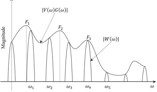
V(ω_k)G(ω_k)W(ω−ω_k, τ) (2.8) Figure 2.3 illustrates the result of the spectral shaping of the main lobe of the window function at the harmonics ω₁, ω₂, . . ., ω_N by the spectral envelope |V(ω)G(ω)| which is

(24)

the contribution from a glottal and vocal tract. The resonance or formants frequencies denoted asF₁,F₂,. . .,F_N, are the peaks of the spectral envelope. According to the above speech production model, there are two classical techniques described in the next section for analyzing speech signals for important parameters relating to the glottal source and vocal tract.

| |

Magnitude

Figure 2.3: Spectral shaping

2.2 Classical techniques

2.2.1 Linear prediction

Linear prediction (LP) is widely used in speech applications such as speech compression because the speech production process is suitable with LP. When the continuous-time speech signal s(t) is sampled by ADC, the result is the discrete time speech signal, s[n], which can be written as

s[k] =

P

X

p=1

a_ps[k−p] +Gu[k], (2.9) where k is the time index, P represents the prediction order, a_p, p = 1, . . . , L, are linear prediction coefficients, G is the gain of the system, and u[k] is the excitation or glottal source signal (sequence). The parameter a_p is a filter coefficient of the vocal-tract on the basis of an all-pole filter model. The vocal tract filter is assumed to be time-invariant within a short duration (20 - 30 ms). Eq. 2.9 can be rewritten in frequency domain by using the z-transform as

V(z) = G

1−PP

p=1a_pz^−p,

= G

A(z), (2.10)

(25)

where V(z) is transfer function of the vocal tract and A(z) its inverse. After obtaining the filter coefficients, the glottal source signal is estimated by using inverse filtering. The details of how to calculate the coefficients of the filter is described as follows. Consider a stationary random signal x[k]. It is assumed that the value of the sample x[k] can be predicted by its past samples, i.e., x[k−1],x[k−2], etc. The prediction error is defined as

e[k] = x[n]−x[k],ˆ

= x[k]−

P

X

p=1

a_px[k−p],

= x[k]−a^Tx[k−1], (2.11)

where the superscript “T” denotes transposition of the matrix, ˆx[k] is the predicted sample, a^T = [a₁ a₂ · · · a_P]^T is a vector of prediction coefficients, and x[k −1] = [x[k−1] x[k −2] · · · x[k−P]]^T is a vector containing the P most recent samples.

To obtain the accurate values of prediction coefficients, it is required to minimize the prediction error by minimizing the mean-square error

J(aP) =E{e²_P[k]}, (2.12)

where E· demotes expectation operator. Differentiate J(a_P) with respect to a_P and equating to 0_{P x1}, i.e.,

R_P a_P =r_P, (2.13)

where

R_P = E{x[k−1]x^T[k−1]},

= E{x[k]x^T[k]},

=







r[0] r[1] · · · r[P −1]

r[1] r[2] · · · r[P −2]

... ... . .. ... r[P −1] r[P −2] · · · r[0]







(2.14)

is the correlation matrix, andr_P is the correlation vector. Assume thatR_P is nonsingular, the optimal prediction coefficients can be calculated by

a_P =R⁻¹_P r_P. (2.15)

Eq. (2.15) can be solved by Levinson-Durbin algorithm [1]. Figure 2.4 illustrates speech analysis using LP where panel (a) is a voiced sound. The prediction coefficients, which are coefficients of vocal tract filter, are calculated by using Matlab function “lpc(·)”. The frequency response of the filter calculated from the coefficients by using Matlab function

“freqz()” is shown as the red line in the panel (b) whereas the blue line is the spectrum of the voiced sound. The glottal source signal which is shown in panel (c) can be obtained by using inverse filtering from the calculated correlation coefficients. Notice that the period of the source signal are the same as that of the voiced sound.

(26)

Time (ms)

2 4 6 8 10 12 14 16 18

Amplitude

-2 0 2

Frequency (kHz)

0 1 2 3 4 5 6 7 8

Magnitude (dB) _-200

-100 0 100

Time (ms)

2 4 6 8 10 12 14 16 18

Amplitude ₀

0.5 1

(a)

(b)

(c)

Figure 2.4: Demostration of speech analysis using LP

2.2.2 Cepstrum

Another technique is the CEP which transforms log magnitude spectrum of a speech signal cepstrum by using the inverse discrete-time Fourier transform (IDFT). That is for a discrete time speech signal s(t), its cepstrum is defined as

c(˜t) = 1 2π

Z π

−π

log|S(ω)|e^jω^˜^tdω (2.16)

where S(ω) is the discrete-time Fourier transform (DTFT) of s(t) which is defined as S(ω) =

Z ∞ n=−∞

s(t)e^−jωtdt. (2.17)

Eq. 2.16 takes only the magnitude spectrum|S(ω)| so that c(˜t) is real like s(t). Consider the same speech signal as shown in Fig. 2.4. According to Eq. (2.2), its cepstrum is

<{F⁻¹[log|S(ω)|]} = <{F⁻¹[log|U(ω)|] +F⁻¹[log|V(ω)|],}

c(˜t) = c_src(˜t) +c_flt(˜t), (2.18) where F⁻¹[·] is the IDTFT, < denotes the real part. Notice that cepstrum of speech consists of cepstrum of the glottal source and vocal tract. Fig. 2.5 shows cepstrum of the voiced sound of Fig. 2.4. c_src(˜t) can be noticed as the peaks in high quefrency range.

(27)

These peak associated withF0 of the speech signal. On the other hand, cflt(˜t) is the peak in low frequency range. These cepstra can be separated using a lifter as shown in the red line in the top panel of Fig. 2.5. After applying the lifter, DTFT of the liftered cepstrum results in spectral envelope, the red line in the bottom panel of Fig. 2.5 where the dashed line is the spectral envelope obtained by using LP. Notice the similar peaks of two spectral envelop.

Quefrency (ms)

1 2 3 4 5 6 7 8 9

Amplitude Cepstrum _-10 -5 0 5 10

Frequency (kHz)

0 1 2 3 4 5 6 7 8

Magnitude (dB)

-150 -100 -50 0 50 100

F0 lifter

Figure 2.5: Demostration of speech analysis using CEP

Complex cepstrum

When both magnitude and phase are taken into consideration, the result will be complex cepstrum of S(ω) that is

logS(ω) = log|S(ω)|+j∠S(ω), (2.19) C(˜ˆ t) = 1

2π Z π

−π

logS(ω)e^jω^˜^tdω (2.20) where ∠S(ω) is phase spectrum of S(ω). t˜is the independent variable in quefrency domain. The relationship between the cepstrum and complex cepstrum can be obtained by

c(˜t) = Even{C(˜ˆ t)}=

C(˜ˆ t) + ˆC(−˜t)

2 (2.21)

(28)

In fact, complex cepstrum can be written in three forms besides Eq. (2.20). They will be used for solving speech analysis in reverberant environments. Therefore, the background knowledge about the complex cepstrum will be written in this subsection. From Eq.

(2.17), S(ω) can be written in polar form as S(ω) = |S(ω)|exp^j∠S(ω),

= |U(ω)||V(ω)|exp^j{^{∠U(ω)+∠V}^(ω)}, (2.22) where ∠U(ω) and ∠V(ω) are phase spectrum. The first form of complex cepstrum of S(ω) is expressed by

C(˜ˆ t) = Cˆ_A(˜t) + ˆC_φ(˜t),

= F⁻¹[log{|S(ω)|exp^j∠S(ω)}],

= F⁻¹[log|S(ω)|] +F⁻¹[j∠S(ω)], (2.23) whereF⁻¹[·] denotes the IDTFT, ˆC_A(˜t) and ˆC_φ(˜t) are the amplitude and phase cepstra. ˜t is an independent variable in quefrency domain having the unit of time. The second form of complex cepstrum of S(ω) is written as

Cˆ_S(˜t) = F⁻¹[logV(ω)] +F⁻¹[logU(ω)],

= CˆS,flt(˜t) + ˆCS,src(˜t), (2.24)

where ˆCsrc(˜t) is the complex cepstrum of the glottal source and ˆCflt(˜t) is of the vocal tract filter. The third form of complex cepstrum ofS(ω) is represented by summation of non-minimum and minimum phase components. That is

Cˆ_S(˜t) = Cˆ_S,min(˜t) + ˆC_S,all(˜t),

= Cˆ_S,A,min(˜t) + ˆC_S,φ,min(˜t)

+ ˆC_S,A,all(˜t) + ˆC_S,φ,all(˜t), (2.25) where the subscripts “all” and “min” denote non-minimum phase and minimum components. In fact, the clean speech spectra can also be represented as

S(ω) = S_min(ω)S_all(ω),

= |S_min(ω)|exp^jφ^min|S_all(ω)|exp^jφ^all. (2.26) Since |S_all(ω)| = 1. Thus, ˆC_S,φ,all(˜t) = 0. Therefore, there are remaining three components of complex cepstrum. Speech dereverberation by using complex cepstrum analyisis, described in Chapter 5, is also on the basis of this fact. In reverberant environments, a reverberant speech signal, y(t), is defined as

y(t) =s(t)∗h(t), (2.27)

whereh(t) is the room impulse response (RIR). The Fourier transform ofy(t) is expressed as

Y(ω) = S(ω)H(ω),

= U(ω)V(ω)H(ω), (2.28)

(29)

whereH(ω) is the Fourier transform of the RIR. The complex cepstrum of the reverberant speech signal is

Cˆ_Y(˜t) = ˆC_S,src(˜t) + ˆC_S,flt(˜t) + ˆC_H(˜t), (2.29) where ˆC_H(˜t) is the complex cepstrum of the RIR. As a result, ˆC_Y(˜t) is separately represented as

Cˆ_Y(˜t) = Cˆ_Y,A,min(˜t) + ˆC_Y,φ,min(˜t) + ˆC_Y,φ,all(˜t),

= CˆS,src,A,min(˜t) + ˆCS,src,φ,min(˜t) + ˆCS,src,φ,all(˜t) + ˆCS,flt,A,min(˜t) + ˆCS,flt,φ,min(˜t) + ˆCS,flt,φ,all(˜t), + ˆC_H,A,min(˜t) + ˆC_H,φ,min(˜t)

+ ˆC_H,φ,all(˜t). (2.30)

In the calculation, the minimum phase component is extracted from the amplitude cepstrum. That is

CˆY,A,min(˜t) = CY(˜t)·L(˜t), (2.31) Cˆ_Y,φ,min(˜t) = Cˆ_Y,A,min−C_Y(˜t), (2.32) whereL(˜t) is the appropriate lifter (Oppenheim and Schafer, 2009). Since|Yall(ω, τ)|= 1.

Thus ˆC_Y,A,all(˜t) = 0. Therefore, ˆC_Y,φ,all(˜t) can be extracted by subtracting the above minimum phase cepstra from Eq. (2.30). On important notation is that ˆC_Y,A,min(˜t) is similar to ˆC_Y,φ,min(˜t) within a certain range of quefrency. This notation is useful to estimate both of them from ˆC_Y(˜t)

2.3 Empirical mode decomposition and its extensions

To date, several powerful data analysis approaches are available such as Fourier spectral analysis, wavelet analysis, and singular value decomposition (SVD) based analysis. These still have limitations in several cases. Fourier spectral analysis as shown in previous subsections has been dominated in time-frequency analysis of signals for a long time.

It has been a general method for globally examining the energy-frequency distributions within a specified range of time such as spectrogram. However, there are some critical limitations of the Fourier analysis which are (i) the system must be linear, and (ii) the data must be strictly periodic or stationary. Its failures are usually caused by in sufficient spanning, non-stationary, and non-linearity of the data.

Wavelet analysis is an alternative linear analysis for non-stationary data analysis.

Its limitations are caused by the selection of basic wavelet function. Once the basic wavelet is selected, one will have to use it to analyze all the data which is its non-adaptive nature. Singular value decomposition (SVD), also known as empirical orthogonal function expansion or principal component analysis, is another well-known data analysis tool. SVD provides only a distribution of the oscillating mode by using the variance defined by eigenvalues. This distribution does not inform frequency content of the signal. Moreover, it is difficult the define the physical meaning of a single component of the decomposition.

Recently, Huang et al [9] proposed a new data analysis method namely empirical mode decomposition (EMD) which directly extracts the energy associated with various intrinsic

(30)

time scales into intrinsic mode functions (IMFs). EMD does not assume that the process must be linear or stationary. The IMFs are derived from the data that serves as the basis expansion regardless the linearity of the data. In other words, EMD is data driven and adaptive analysis approach. The full energy distribution on the time-frequency scale is derived from the local energy and the instantaneous frequency (IF) through the Hilbert transform, i.e. Hilbert spectrum.

2.3.1 Iterarive algorithm of EMD

EMD decomposes a signal x(t) into IMFs by using its extrema. Thus the signal must have at least one maximum and one minimum. The time between these extrema is defined as the characteristic time scale. The sifting process for extracting IMFs is described as follows.

1. Locate all extrema of the input signal x(t).

2. Connect all maxima by using a cubic spline interpolation as the upper envelope and do the same fo all minima to make the lower envelope.

3. The mean between the upper and lower envelopes is designated as m(t). Let the IMF candidate be d(t) =x(t)−m(t).

4. If d(t) is IMF, it should be symmetric: the number of extrema differs from the number of zero crossings at most by one and the mean defined by the difference between its upper and lower envelope is zero. Otherwise, d(t) will be treated as input data and fed into the sifting process (1)-(3) for more i rounds until the IMF candidate d(t) fulfills the properties of IMF. Otherwise go to the next step.

5. The first IMF of x(t) is extracted by as q₁(t) = x(t)−d(t). The residue which is defined as r₁(t) = x(t)−q₁(t) will be treated as input data for extracting other IMFs by feeding into the sifting process (1)-(4).

6. After K IMFs are extracted and the energy of r_K(t) is very small or a monotonic function, the sifting process stops.

After decomposing x(t) by the sifting process, x(t) can be reconstructed by summing all IMFs and residue, i.e.,

x(t) =

K

X

k=1

qk(t) +rK(t), (2.33)

where K is the number of IMFs, q_k(t) is the k-th IMF, and r_K(t) is residue. The zero mean of IMF is indicated by the small value of the standard deviation which is defined by standard deviation of d(t) of previous round, d_i−1(t), and the current round, d_i(t), [9].

That is

SD =

T

X

t=1

|di−1(t)−d_i(t)|²

d²_i−1(t) . (2.34)

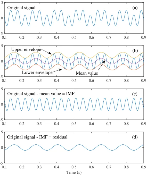
A typical value for SD is between 0.2 and 0.3 calculated from the data having 1024 points. Another criterion stops the sifting process when d_i(t) has an insufficient number of extrema [24] indicating the oscillatory component. The demonstration of the sifting

(31)

process is shown in Fig. 2.6 where the original signal is shown in panel (a). Panel (b) shows the upper and lower envelopes constructed from the extrema which can be observed by eyes. The mean is the difference between the upper and lower envelopes. Panel (c) shows the difference between the original signal in panel (a) and the mean in panel (b) which, fortunately, is the first IMF. Panel (d) is r₁(t) which will be further decomposed the remaining IMFs.

0.1 0.2 0.3 0.4 0.5 0.6 0.7 0.8 0.9

-5 0 5

0.1 0.2 0.3 0.4 0.5 0.6 0.7 0.8 0.9

-5 0 5

0.1 0.2 0.3 0.4 0.5 0.6 0.7 0.8 0.9

-5 0 5

Time (s)

0.1 0.2 0.3 0.4 0.5 0.6 0.7 0.8 0.9

-5 0 5

(a)

(c) (b)

(d) Upper envelope

Lower envelope Mean value Original signal

Original signal - mean value = IMF

Original signal - IMF = residual

Figure 2.6: Demonstration of sifting process

To date, several extensions of EMD have been developed to eliminate its weak points and to make suitable for several applications relating to data fusion from multiple sources.

Three major extensions are bivariate EMD [25], trivariate EMD [26], and multivariate EMD (MEMD) [27]. Bivariate EMD (BEMD) originated from complex EMD (CEMD), applying EMD to complex numbers, and rotation-invariant EMD (RI-EMD), more general realization of the complex EMD that designates fast oscillating as fast rotating compo-

(32)

nents and slow oscillating as slow rotating components. Trivariate EMD (TEMD) extends the concept of extracting fast and slow rotating components by using Quaternion algebra which is more appropriate for the rotation in 3D space. The most current extension is the multivariate EMD (MEMD) which allows more fusion of the data from several sources such as multiple sensors. The important property of these extensions of EMD is the common mode alignment which is exploited frequently in our proposed speech analysis method.

2.3.2 Bivariate EMD

The basic concept of EMD is “univariate signal is equal to fast oscillations added on slower oscillations” whereas the basic idea of BEMD is “bivariate signal is equivalent to fast rotations added on slower rotations.” The bivariate signal can be formed by using two time series signals with the same length. Consider Fig. 2.7 where a bivariate signal is in panel (a). The envelope of the bivariate signal is shown in panel (b). Its IMFs are two component of oscillations as shown in panel (c) and (d).

Figure 2.7: Demonstration of bivariate EMD

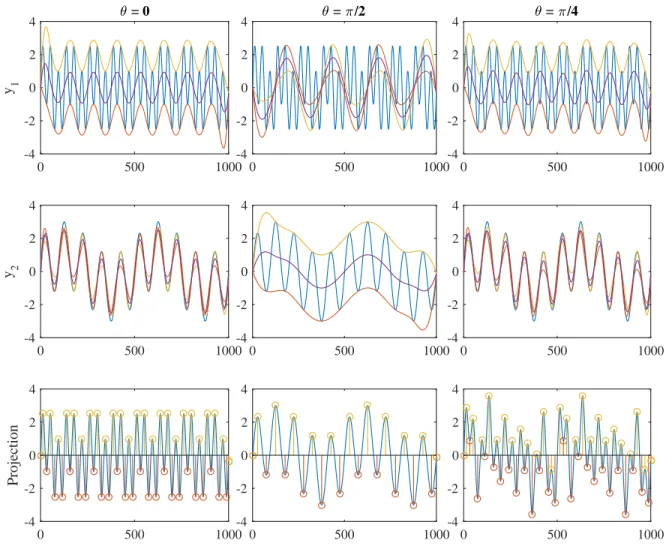
Rather than decomposing each time series individually by using EMD, two time series can be jointly decomposed by using BEMD. The example is given as follows. Consider two time series y₁ and y₂ represented by the blue lines in Fig. 2.8. A direction vector is defined by using the angleθrelative to the +x-axis. The projections ofy1and y2 based on three values of θ are the blue lines in the bottom panels. The upper and lower envelopes of y₁ and y₂ are calculated by using the time instances of extrema of projections in the corresponding column. Note that when θ = 0, the projection is equal to y1 and equal to y₂ when θ = π/2. There are three mean time series, represented by the purple lines in

(33)

Fig. 2.8, according to three values of θ. The average from these mean time series is used to extract an IMF.

0 500 1000

y 1

-4 -2 0 2

4 3 = 0

0 500 1000

y 2

-4 -2 0 2 4

0 500 1000

Projection

-4 -2 0 2 4

0 500 1000

-4 -2 0 2

4 3 = :/2

0 500 1000

-4 -2 0 2 4

0 500 1000

-4 -2 0 2 4

0 500 1000

-4 -2 0 2

4 3 = :/4

0 500 1000

-4 -2 0 2 4

0 500 1000

-4 -2 0 2 4

Figure 2.8: Example extrema of bivariate signal at a given instant in time

A more general approach is described as follows. Assume that bivariate signal is in the form of complex-valued signal. Let a set of directions be θ_k = 2kπ/N,1 < k < N where N is the number of directions on 2D space. An IMF is extracted by

1. Project the complexed-valued signal x(t) on direction θ_k:

2. p_θ_k(t) = <{e^−iθ^kx(t)}where<denotes the real part of the complexed-valued signal.

3. Extract the locations {t^k_j} of the extrema of p_θ_k(t).

4. Interpolate the set {t^k_j}, x[{t^k_j}] to obtain the upper and lower envelope curves and their mean m_θ_k(t). Repeat step (1)-(4) again for allN directions.

5. The mean of all envelope curves is computed by: m(t) = _N¹ PN

k=1m_θ_k(t). Note that m(t) is also a complex time series.

6. The mean is subtracted from x(t) by: d(t) = x(t)−m(t).

(34)

These steps are the same as steps (1)-(4) of univariate EMD described earlier. The remaining process are the same for extracting IMFs. There are other similar algorithms for extracting IMFs from a bivariate signal which can be found in [25]. Only, the simplest one is described in here. The important concept of BEMD is the projection of the input signal on an directional axis which will be frequency used in other two extensions of EMD.

2.3.3 Trivariate EMD

The important concept of BEMD is that it utilizes the projections of the bivariate signal in multiple directions to find the local extrema. This concept can also be applied when the dimension is more than two. Furthermore, rather than using normal 3D projection in 3D space, the trivariate EMD employs a quaternion rotation for the projection in 3D space as follows.

A B

u ϕ r’ r

Figure 2.9: Rotation of a vector r around a unit vector u or line segmentABby and angle φ.

Let o=a+b¯i+cj¯+dk¯ be a quaternion where a,b, c, and d are real numbers and ¯i,

¯j, and ¯k are the unit vectors along +x, +y, and +z-axis. The important notation is the so-called unit quaternion which is written as

o = cosφ+usinφ (2.35)

= e^uφ, (2.36)

where u is a 3D unit vector. Eq. (2.36) is the generalization of Euler’s identity that represents the rotation of a vector by an angle 2φ about a 3D unit vector u as shown in Fig. 2.9. This figure demonstrates the rotation of a vector rby an angle φabout the line segment AB. The direction of AB is specified by a 3D unit vector u, and the rotated vector is represented by r⁰, that is

r⁰ =oro^∗ =e^uφ/2r(e^uφ/2)^∗, (2.37)